Limitations of Algorithm Power.

Limitations of Algorithm Power

Objectives

We now move into the third and final major theme for this course.

1. Tools for analyzing algorithms.

2. Design strategies for designing algorithms.

3. Identifying and coping with the limitations of algorithms.

Efficiency of an algorithm

• By establishing the asymptotic efficiency class

• The efficiency class for selection sort (quadratic) is lower. Does this mean that selection sort is a “better” algorithm?

– Like comparing “apples” to “oranges”

• By analyzing how efficient a particular algorithm is compared to other algorithms for the same problem

– It is desirable to know the best possible efficiency any algorithm solving this problem may have – establishing a lower bound

Lower Bounds

Lower bound: an estimate on a minimum amount of work needed to solve a given problem

Examples:

• number of comparisons needed to find the largest element in a set of n numbers

• number of comparisons needed to sort an array of size n

• number of comparisons necessary for searching in a sorted array

• number of multiplications needed to multiply two n-by-n matrices Lower bound can be

– an exact count

– an efficiency class (Ω)

• Tight lower bound: there exists an algorithm with the same efficiency as the lower bound

Methods for Establishing Lower Bounds

• trivial lower bounds

• information-theoretic arguments (decision trees)

• adversary arguments

• problem reduction

Trivial Lower Bounds

Trivial lower bounds: based on counting the number of items that must be processed in input and generated as output Examples

• finding max element

• polynomial evaluation

• sorting

• element uniqueness

• computing the product of two n-by-n matrices

Conclusions

• may and may not be useful

• be careful in deciding how many elements must be processed

Decision Trees

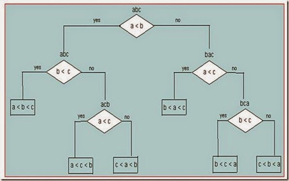
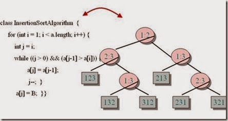
Decision tree — a convenient model of algorithms involving Comparisons in which: (i) internal nodes represent comparisons (ii) leaves represent outcomes Decision tree for 3-element insertion sort

Deriving a Lower Bound from Decision Trees

• How does such a tree help us find lower bounds?

– There must be at least one leaf for each correct output.

– The tree must be tall enough to have that many leaves.

• In a binary tree with l leaves and height h,

h ≥ llog2 ll

Decision Tree and Sorting Algorithms

Decision Tree and Sorting Algorithms

• Number of leaves (outcomes) ≥ n!

• Height of binary tree with n! leaves ≥ log2n!

• Minimum number of comparisons in the worst case ≥ log2n! for any comparison-based sorting algorithm

• log2n! ≈ n log2n

• This lower bound is tight (e.g. mergesort)

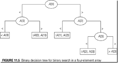
Decision Tree and Searching a Sorted Array

Decision Tree and Searching a Sorted Array

• Number of leaves (outcomes) = n + n+1 = 2n+1

• Height of ternary tree with 2n+1 leaves ≥ log3 (2n+1)

• This lower bound is NOT tight (the number of worst-case comparisons for binary search is  log2 (n+1) , and  log3 (2n+1) ≤ log2 (n+1)

• Can we find a better lower bound or find an algorithm with better efficiency than binary search?

Decision Tree and Searching a Sorted Array

Decision Tree and Searching a Sorted Array

• Consider using a binary tree where internal nodes also serve as successful searches and leaves only represent unsuccessful searches

• Number of leaves (outcomes) = n + 1

• Height of binary tree with n+1 leaves ≥ log2 (n+1)

• This lower bound is tight

Decision-tree model

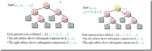
A decision tree can model the execution of any comparison sort:

• One tree for each input size n.

• View the algorithm as splitting whenever it compares two elements.

• The tree contains the comparisons along all possible instruction traces.

• The running time of the algorithm = the length of the path taken.

• Worst-case running time = height of tree.

Any comparison sort can be turned into a Decision tree

Decision Tree Model

• In the insertion sort example, the decision tree reveals all possible key comparison sequences for 3 distinct numbers.

• There are exactly 3!=6 possible output sequences.

• Different comparison sorts should generate different decision trees.

• It should be clear that, in theory, we should be able to draw a decision tree for ANY comparison sort algorithm.

• Given a particular input sequence, the path from root to the leaf path traces a particular key comparison sequence performed by that comparison sort.

- The length of that path represented the number of key comparisons performed by the sorting algorithm.

• When we come to a leaf, the sorting algorithm has determined the sorted order.

• Notice that a correct sorting algorithm should be able to sort EVERY possible output sorted order.

• Since, there are n! possible sorted order, there are n! leaves in the decision tree.

• Given a decision tree, the height of the tree represent the longest length of a root to leaf path.

• It follows the height of the decision tree represents the largest number of key comparisons, which is the worst-case running time of the sorting algorithm.

“Any comparison based sorting algorithm takes Ω(n logn) to sort a list of n distinct elements in the worst-case.”

• We want to find a lower bound (Ω) of the height of a binary tree that has n! Leaves.

◊ What is the minimum height of a binary tree that has n! leaves?

• The binary tree must be a complete tree (recall the definition of complete tree).

• Hence the minimum (lower bound) height is θ(log2(n!)).

• log2(n!)

= log2(n) + log2(n-1) + …+ log2(n/2)+….

≥ n/2 log2(n/2) = n/2 log2(n) – n/2

So, log2(n!) = Ω(n logn).

• It follows the height of a binary tree which has n! leaves is at least Ω(n logn) ◊ worst- case running time is at least Ω(n logn)

• Putting everything together, we have

“Any comparison based sorting algorithm takes Ω(n logn) to sort a list of n distinct elements in the worst-case.”

Adversary Arguments

Adversary argument: a method of proving a lower bound by playing role of adversary that makes algorithm work the hardest by adjusting input Example: “Guessing” a number between 1 and n with yes/no questions Adversary: Puts the number in a larger of the two subsets generated by last question

Lower Bounds by Problem Reduction

Idea: If problem P is at least as hard as problem Q, then a lower bound for Q is also a lower bound for P.

Hence, find problem Q with a known lower bound that can be reduced to problem P in question.

Example: Euclidean MST problem

• Given a set of n points in the plane, construct a tree with minimum total length that connects the given points. (considered as problem P)

• To get a lower bound for this problem, reduce the element uniqueness problem to it. (considered as problem Q)

• If an algorithm faster than n log n exists for Euclidean MST, then one exists for element uniqueness also. Aha! A contradiction! Therefore, any algorithm for Euclidean MST must take Ω(n log n) time.

Classifying Problem Complexity

Is the problem tractable, i.e., is there a polynomial-time (O(p(n)) algorithm that solves it?

Possible answers:

• yes (give examples)

• no

– because it’s been proved that no algorithm exists at all (e.g., Turing’s halting problem)

– because it’s been proved that any algorithm for the problem takes exponential time

• unknown

Problem Types: Optimization and Decision

• Optimization problem: find a solution that maximizes or minimizes some objective function

• Decision problem: answer yes/no to a question

Many problems have decision and optimization versions.

E.g.: traveling salesman problem

• optimization: find Hamiltonian cycle of minimum length

• decision: find Hamiltonian cycle of length ≤ m

Decision problems are more convenient for formal investigation of their complexity.

Class P

P: the class of decision problems that are solvable in O(p(n)) time, where p(n) is a polynomial of problem’s input size n

Examples:

• searching

• element uniqueness

• graph connectivity

• graph acyclicity

• primality testing (finally proved in 2002)

Class NP

NP (nondeterministic polynomial): class of decision problems whose proposed solutions can be verified in polynomial time = solvable by a nondeterministic polynomial algorithm

A nondeterministic polynomial algorithm is an abstract two-stage procedure that:

• generates a random string purported to solve the problem

• checks whether this solution is correct in polynomial time

By definition, it solves the problem if it’s capable of generating and verifying a solution on one of its tries

Why this definition?

• led to development of the rich theory called “computational complexity”

Example: CNF satisfiability

Problem: Is a boolean expression in its conjunctive normal form (CNF) satisfiable, i.e., are there values of its variables that makes it true?

This problem is in NP. Nondeterministic algorithm:

• Guess truth assignment

• Substitute the values into the CNF formula to see if it evaluates to true

What problems are in NP?

• Hamiltonian circuit existence

• Partition problem: Is it possible to partition a set of n integers into two disjoint subsets with the same sum?

• Decision versions of TSP, knapsack problem, graph coloring, and many other combinatorial optimization problems. (Few exceptions include: MST, shortest paths)

• All the problems in P can also be solved in this manner (but no guessing is necessary), so we have:

P ⊆ NP

• Big question: P = NP ?

P = NP ?

• One of the most important unsolved problems is computer science is whether or not

P=NP.

– If P=NP, then a ridiculous number of problems currently believed to be very difficult will turn out have efficient algorithms.

– If P≠NP, then those problems definitely do not have polynomial time solutions.

• Most computer scientists suspect that P ≠ NP. These suspicions are based partly on the idea of NP-completeness.

NP-Complete Problems

A decision problem D is NP-complete if it’s as hard as any problem in NP, i.e.,

• D is in NP

• every problem in NP is polynomial-time reducible to D

Examples: TSP, knapsack, partition, graph-coloring and hundreds of other problems of combinatorial nature

is it possible to assign the input x1...x9, so that the formula evaluates to TRUE?

- If the answer is YES with a proof (i.e. an assignment of input value), then we can check the proof in polynomial time (SAT is in NP)

- We may not be able to check the NO answer in polynomial time (Nobody really knows.)

• NP-hard

- A problem is NP-hard iff an polynomial-time algorithm for it implies a polynomial- time algorithm for every problem in NP

- NP-hard problems are at least as hard as NP problems

• NP-complete

- A problem is NP-complete if it is NP-hard, and is an element of NP (NP-easy)

• Relationship between decision problems and optimization problems

- every optimization problem has a corresponding decision problem

- optimization: minimize x, subject to constraints

- yes/no: is there a solution, such that x is less than c?

- an optimization problem is NP-hard (NP-complete)

if its corresponding decision problem is NP-hard (NP-complete)

• How to know another problem, A, is NP-complete?

- To prove that A is NP-complete, reduce a known NP-complete problem to A

• Requirement for Reduction

-Polynomial time

-YES to A also implies YES to SAT, while

NO to A also implies No to SAT

Examples of NP-complete problems

Vertex cover

• Vertex cover

- given a graph G=(V,E), find the smallest number of vertexes that cover each edge

- Decision problem: is the graph has a vertex cover of size K?

• Independent set

- independent set: a set of vertices in the graph with no edges between each pair of nodes.

- given a graph G=(V,E), find the largest independent set

- reduction from vertex cover:

• Set cover

- given a universal set U, and several subsets S1,...Sn

- find the least number of subsets that contains each elements in the universal set

Polynomial (P) Problems

• Are solvable in polynomial time

• Are solvable in O(nk), where k is some constant.

• Most of the algorithms we have covered are in P

Nondeterministic Polynomial (NP) Problems

• This class of problems has solutions that are verifiable in polynomial time.

– Thus any problem in P is also NP, since we would be able to solve it in polynomial time, we can also verify it in polynomial time

NP-Complete Problems

• Is an NP-Problem

• Is at least as difficult as an NP problem (is reducible to it)

• More formally, a decision problem C is NP-Complete if:

– C is in NP

– Any known NP-hard (or complete) problem ≤p C

– Thus a proof must show these two being satisfied

Exponential Time Algorithms

Examples

• Longest path problem: (similar to Shortest path problem, which requires polynomial

time) suspected to require exponential time, since there is no known polynomial algorithm.

• Hamiltonian Cycle problem: Traverses all vertices exactly once and form a cycle.

Reduction

• P1 : is an unknown problem (easy/hard ?)

• P2 : is known to be difficult

If we can easily solve P2 using P1 as a subroutine then P1 is difficult Must create the inputs for P1 in polynomial time.

* P1 is definitely difficult because you know you cannot solve P2 in polynomial time unless you use a component that is also difficult (it cannot be the mapping since the mapping is known to be polynomial)

Decision Problems

• Represent problem as a decision with a boolean output

– Easier to solve when comparing to other problems

– Hence all problems are converted to decision problems. P = {all decision problems that can be solved in polynomial time}

NP = {all decision problems where a solution is proposed, can be verified in polynomial time}

NP-complete: the subset of NP which are the “hardest problems”

Alternative Representation

• Every element p in P1 can map to an element q in P2 such that p is true (decision

problem) if and only if q is also true.

• Must find a mapping for such true elements in P1 and P2, as well as for false elements.

• Ensure that mapping can be done in polynomial time.

• *Note: P1 is unknown, P2 is difficult

Cook’s Theorem

• Stephen Cook (Turing award winner) found the first NP-Complete problem, 3SAT.

• Basically a problem from Logic.

• Generally described using Boolean formula.

• A Boolean formula involves AND, OR, NOT operators and some variables.

Ex: (x or y) and (x or z), where x, y, z are boolean variables.

• Problem Definition – Given a boolean formula of m clauses, each containing ‘n’ boolean variables, can you assign some values to these variables so that the formula can be true?

• Boolean formula: (x v y v z) Λ (x v y v z)

• Try all sets of solutions. Thus we have exponential set of possible solutions. So it is a NPC problem.

• Having one definite NP-Complete problem means others can also be proven NP- Complete, using reduction.