B Trees:The B+-tree

The B+-tree

The most well-know variation of the B-tree is the B+-tree. There are two major differences from the B-tree. First, all objects in the B+-tree are kept in leaf nodes. Second, all leaf nodes are linked together as a double-linked list.

The structure of the B+-tree looks quite similar to the B-tree. Thus we omit the details. We do point out that in an index node of a B+-tree, different from the B-tree, we do not store object values. We still store object keys, though. However, since all objects are stored in the leaf level, the keys stored in index nodes act as routers, as they direct the search algorithm to go to the correct child node at each level.

Copy-up and Push-up

One may wonder where the routers in the index nodes come from. To understand this, let’s look at an example. Initially, the B+-tree has a single node which is a leaf node. After 2B insertions, the root node becomes full.

In Figure 15.7(a), if we try to insert an object to the node A when it is already full, it temporarily overflows. To handle the overflow, the B+-tree will split the node into two nodes A and B. Furthermore, a new node C is generated, which is the new root of the tree. The first key in leaf node B is copied up to C. The result B+-tree is shown in Figure 15.7(b).

We point out that a key in an index node may be validly replaced by some other keys, unlike in a leaf node. For instance, in node C of Figure 15.7(b), we can replace the key 40 to 35. As long as it is smaller than all keys in the left sub-tree and bigger than or equal to all keys in the right sub-tree, it is fine.

To emphasize the fact that the keys in a index node are different from the keys in a leaf node (a key in an index node is not a real object), in the B+-tree figures we will attach a (*) to each key in a leaf node.

As a comparison, consider the split of an index node. In Figure 15.8(a), the index node C temporarily overflows. It is split into two, C and G. Since before the split, C was the tree root, a new root node H is generated. See Figure 15.8(b). Here the middle key 51 in the original node C is pushed up to the parent node.

B+-tree Query

As in the B-tree, the B+-tree supports the exact-match query which finds the object with a given key. Furthermore, the B+-tree can efficiently support the range query, which finds the objects whose keys are in a given range.

To perform the exact-match query, the B+-tree follows a single path from root to leaf. In the root node, there is a single child pointer whose key range contains the key to be searched for. If we follow the child pointer to the corresponding child node, inside the child node there is also a single child pointer whose key range contains the object to be searched for. Eventually, we reach a leaf node. The object to be searched, if it exists, must be located in this node. As an example, Figure 15.9 shows the search path if we search key=42.

Beside the exact-match query, the B+-tree also supports the range query. That is, find all objects whose keys belong to a range R. In order to do so, all the leaf nodes of a B+-tree are linked together. If we want to search for all objects whose keys are in the range R =[low, high], we perform an exact match query for key=low. This leads us to a leaf node l. We examine all objects in l, and then we follow the sibling link to the next leaf node, and so on. The algorithm stops when an object with key> high is met. An example is shown in Figure 15.10.

FIGURE 15.10: Illustration of the range query algorithm in the B+-tree. To search for all objects with keys in the range [42,75], the first step is to follow a path from root to leaf to find key 42 (H, C and B are examined). The second step is to follow the right-sibling pointers between leaf nodes and examine D, E. The algorithm stops at E as an object with key=76 is found.

B+-tree Insertion

Since all objects in the B+-tree are located at the leaf level, the insertion algorithm of the B+-tree is actually easier than that in the B-tree. We basically follow the exact-match query to find the leaf node which should contain the object if it were in the tree. Then we insert the object into the leaf node.

What needs to be taken care of is when the leaf node overflows and is split into two. In this case, a key and a child pointer are inserted into the parent node. This may in turn cause the parent node to overflow, and so on. In the worst case, all nodes along the insertion path are split. If the root node splits into two, the height of the tree increases by one. The insertion algorithm is given below.

Algorithm Insert(root, k, v)

Input: the root pageID of a B+-tree, the key k and the value v of a new object.

Prerequisite: the object with key=k does not exist in the tree.

Action: Insert the new object into the B+-tree.

As an example, Figure 15.11 shows how to insert an object with key=60 into the B+-tree shown in Figure 15.9.

B+-tree Deletion

To delete an object from the B+-tree, we first examine a single path from root to the leaf node containing the object. Then we remove the object from the node. At this point, if the node is at least half full, the algorithm returns. Otherwise, the algorithm tries to re-distribute objects between a sibling node and the underflowing node. If redistribution is not possible, the underflowing node is merged with a sibling.

Algorithm Delete(root, k)

Input: the root pageID of a B+-tree, the key k of the object to be deleted.

Prerequisite: the object with key=k exists in the tree.

Action: Delete the object with key=k from the B+-tree.

FIGURE 15.11: After inserting an object with key=60 into the B+-tree shown in Figure 15.9. Leaf node D splits into two. The middle key 56 is copied up to the parent node G.

Step 1 of the algorithm follows a single path from root to leaf to find the object to be deleted. Step 2 deletes the object. The algorithm will finish at this point if any of the following two conditions hold. One, if the tree has a single node (step 3). Two, the leaf node is at least half full after the deletion (the while loop of step 4 is skipped).

As an example, suppose we delete object 56 and then 62 from the B+-tree shown in Figure 15.9.

The deletions go to the same leaf node D, where no underflow occurs. The result is shown in Figure 15.12.

Now, let’s try to delete key 53 from Figure 15.12. This time D underflows. Step 4 of the Delete algorithm handles underflows. In general, when a node xi underflows, the algorithm tries to borrow some entries from a sibling node s, as described in step 4(a). Note that we could borrow just one entry to avoid underflow in xi. However, this is not good because next time we delete something from xi, it will underflow again. Instead, the algorithm redistribute entries evenly between xi and s. Assume xi has B − 1 objects and s has B + k objects, where k ∈ [1..B]. After redistribution, both xi and s will have B + (k − 1)/2 objects. Thus xi can take another (k − 1)/2 deletions before another underflow occurs.

In our example, to delete key 53 from node D, we re-distribute objects in D and E, by moving 72* into D. As discussed in step 4(a)ii of the algorithm, we also needs to modify a key in the parent node G. In our case, since D is a leaf node, we simply replace the key 72 by 75 in node G. Here 75 is the smallest key in E. The result after the redistribution is shown in Figure 15.13. As a comparison, consider the hypothetical case when D were an index node. In this case, we would drag down the key 72 from G to D and push up a key from E to G.

Let’s proceed the example further by deleting object 72 from the tree in Figure 15.13. Now, the node D underflows, and redistribution is not possible (since E, the only immediate sibling of D, is exactly half full). Step 4(b) of the Delete algorithm tells us to merge D and E together. Correspondingly, a key and a child pointer need to be deleted from the parent node G. Since D is a leaf node, we simply delete the key 75 and the child pointer from G. The result is shown in Figure 15.14. As a comparison, imagine D were an index node. We would still remove key 75 and the child pointer from G, but we would keep the key 75 in node D.

One may wonder why in the redistribution and the merge algorithms, the leaf node and the index node are treated differently. The reason is because when we generated an index entry, we had treated two cases differently: the case when the entry points to a leaf node and the case when the entry points to a index node. This is discussed at the beginning of Section 15.4. To generate a new entry pointing to a leaf node, we copied the smallest key from the leaf node. But to generate a new entry pointing to an index node, we pushed a key from the child node up. A key which was copied up can be safely deleted later (when merge occurs). But a key which was pushed up must be kept somewhere. If we delete it from a parent node, we should drag it down to a child node.

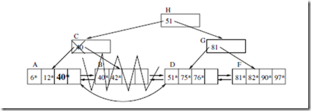
As a running example of merging index nodes, consider deleting object 42 from the B+- tree of Figure 15.14. Node B underflows, and it is merged with A. Correspondingly, in the parent node C, the key 40 and the child pointer to B are deleted. The temporary result is shown in Figure 15.15. It’s temporary since node C underflows.

To handle the underflow of node C, it is merged with G, its sole sibling node. As a consequence, the root node H now has only one child. Thus, H is removed and C becomes the new root. We point out that to merge two index nodes C and G, a key is dragged down from the parent node (versus being deleted in the case of merging leaf nodes). The final

FIGURE 15.15: Temporary tree in the middle of deleting object 42 from Figure 15.14.

Nodes A and B are merged. Key 40 and child pointer to B are removed from C.

FIGURE 15.16: After the deletion of object 42 is finished. This figure illustrates an example of merging two index nodes. In particular, index nodes C and G are merged. The key 51 is dragged down from the parent node H. Since that is the only key in root H, node C becomes the new root and the height of the tree is decreased by one.

result after completing the deletion of 42* is shown in Figure 15.16.