Trees with Minimum Weighted Path Length:Optimal Binary Search Trees.

Optimal Binary Search Trees

Assume we have a sequence of 2n + 1 weights (nonnegative reals)

α0, β1, α1, β2,..., αn−1, βn, αn.

Let Tree(α0, β1, α1, β2,..., αn−1, βn, αn) be the set of all full binary weighted trees with n internal nodes, where the i-th internal node (in the in-order) has the weight βi, and the i-th external node (the leaf, in the left-to-right order) has the weight αi. The in-order traversal results if we visit all nodes in a recursive way, first the left subtree, then the root, and afterwards the right subtree.

If T is a binary search tree then define the cost of T as follows:

Let OP T (α0, β1,..., αn−1, βn, αn) be the set of trees Tree(α0, β1,..., αn−1, βn, αn) whose cost is minimal.

We use also terminology from [35]. Let K1,... Kn be a sequence of n weighted items (keys), which are to be placed in a binary search tree. We are given 2n + 1 weights (probabilities): q0, p1, q1, p2, q2, p3,..., qn−1, pn, qn where

• pi is the probability that Ki is the search argument;

• qi is the probability that the search argument lies between Ki and Ki+1.

The OBST problem is to construct an optimal binary search tree, the keys Ki’s are to be stored in internal nodes of this binary search tree and in its external nodes special items are to be stored. The i-th special item Kt corresponds to all keys which are strictly between Ki and Ki+1. The binary search tree is a full binary tree whose nodes are labeled by the keys.

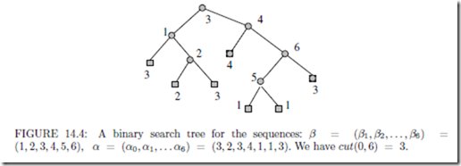
Using the abstract terminology introduced above the OBST problem consists of finding a tree T ∈ OP T (q0, p1, q1, p2,... , qn−1, pn, qn), see an example tree in Figure 14.4.

Denote by obst(i, j) the set OP T (qi, pi+1, qi+1,..., qj−1, pj , qj ). Let cost(i, j) be the cost of a tree in obst(i, j), for i< j, and cost(i, i) = qi. The sequence qi, pi+1, qi+1,..., qj−1, pj , qj is here the subsequence of q0, p1, q1, p2,..., qn−1, pn, qn, consisting of some number of con- secutive elements which starts with qi and ends with qj . Let

The dynamic programming approach to the computation of the OBST problem relies on the fact that the subtrees of an optimal tree are also optimal. If a tree T ∈ obst(i, j) contains in the root an item Kk then its left subtree is in obst(i, k − 1) and its right subtree is in obst(k, j). Moreover, when we join these two subtrees then the contribution of each node increases by one (as one level is added), so the increase is w(i, j). Hence the costs obey the following dynamic programming recurrences for i < j:

Denote the smallest value of k which minimizes the above equation by cut(i, j). This is the first point giving an optimal decomposition of obst(i, j) into two smaller (son) subtrees. Optimal binary search trees have the following crucial property (proved in [34], see the figure for graphical illustration)

The property of monotonicity, the cuts and the quadratic algorithm for the OBST were first given by Knuth. The general dynamic programming recurrences were treated by Yao [52], in the context of reducing cubic time to quadratic.

THEOREM 14.6 Optimal binary search trees can be computed in O(n2) time.

Proof The values of cost(i, j) are computed by tabulating them in an array. Such tabu- lation of costs of smaller subproblems is the basis of the dynamic programming technique. We use the same name cost for this array. It can be computed in O(n3) time, by processing diagonal after diagonal, starting with the central diagonal.

In case of optimal binary search trees this can be reduced to O(n2) using additional

tabulated values of the cuts in table cut. The k-th diagonal consists of entries i, j such that j − i = k. If we have computed cuts for k-th diagonal then for (i, j) on the (k + 1)-th diagonal we know that

which is O(n). Summing over all diagonals gives quadratic total time to compute the tables of cuts and costs. Once the table cost(i, j) is computed then the construction of an optimal tree can be done in quadratic time by tracing back the values of cuts.

Approximately Optimal Binary Search Trees

We can attempt to reduce time complexity at the cost of slightly increased cost of the constructed tree. A common-sense approach would be to insert the keys in the order of decreasing frequencies. However this method occasionally can give quite bad trees.

Another approach would be to choose the root so that the total weights of items in the left and right trees are as close as possible. However it is not so good in pessimistic sense.

The combination of this methods can give quite satisfactory solutions and the resulting algorithm can be linear time, see [44]. Average subquadratic time has been given in [29].