Multidimensional Spatial Data Structures:Bucketing Methods

Bucketing Methods

There are four principal approaches to decomposing the space from which the objects are drawn. The first approach makes use of an object hierarchy and the space decomposition is obtained in an indirect manner as the method propagates the space occupied by the objects up the hierarchy with the identity of the propagated objects being implicit to the hierarchy. In particular, associated with each object is a an object description (e.g., for region data, it is the set of locations in space corresponding to the cells that make up the object). Actually, since this information may be rather voluminous, it is often the case that an approximation of the space occupied by the object is propagated up the hierarchy rather than the collection of individual cells that are spanned by the object. For spatial data, the approximation is usually the minimum bounding rectangle for the object, while for non- spatial data it is simply the hyper rectangle whose sides have lengths equal to the ranges of the values of the attributes. Therefore, associated with each element in the hierarchy is a bounding rectangle corresponding to the union of the bounding rectangles associated with the elements immediately below it.

The R-tree (e.g., [7, 31]) is an example of an object hierarchy which finds use especially in database applications. The number of objects or bounding rectangles that are aggregated in each node is permitted to range between m ≤ IM/2l and M . The root node in an R-tree has at least two entries unless it is a leaf node in which case it has just one entry corresponding to the bounding rectangle of an object. The R-tree is usually built as the objects are encountered rather than waiting until all objects have been input. The hierarchy

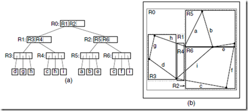
FIGURE 16.6: (a) R-tree for the collection of line segments with m=2 and M=3, in Figure 16.5, and (b) the spatil extents of the bounding rectangles. Notice that the leaf nodes in the index also store bounding rectangles although this is only shown for the nonleaf nodes.

is implemented as a tree structure with grouping being based, in part, on proximity of the objects or bounding rectangles.

For example, consider the collection of line segment objects given in Figure 16.5 shown embedded in a 4 × 4 grid. Figure 16.6a is an example R-tree for this collection with m = 2 and M = 3. Figure 16.6b shows the spatial extent of the bounding rectangles of the nodes in Figure 16.6a, with heavy lines denoting the bounding rectangles corresponding to the leaf nodes, and broken lines denoting the bounding rectangles corresponding to the subtrees rooted at the nonleaf nodes. Note that the R-tree is not unique. Its structure depends heavily on the order in which the individual objects were inserted into (and possibly deleted from) the tree.

Given that each R-tree node can contain a varying number of objects or bounding rectangles, it is not surprising that the R-tree was inspired by the B-tree [6]. Therefore, nodes are viewed as analogous to disk pages. Thus the parameters defining the tree (i.e., m and M ) are chosen so that a small number of nodes is visited during a spatial query (i.e., point and range queries), which means that m and M are usually quite large. The actual implementation of the R-tree is really a B+-tree [18] as the objects are restricted to the leaf nodes.

The efficiency of the R-tree for search operations depends on its ability to distinguish between occupied space and unoccupied space (i.e., coverage), and to prevent a node from being examined needlessly due to a false overlap with other nodes. In other words, we want to minimize coverage and overlap. These goals guide the initial R-tree creation process as well, subject to the previously mentioned constraint that the R-tree is usually built as the objects are encountered rather than waiting until all objects have been input.

The drawback of the R-tree (and any representation based on an object hierarchy) is that it does not result in a disjoint decomposition of space. The problem is that an object is only associated with one bounding rectangle (e.g., line segment i in Figure 16.6 is associated with bounding rectangle R5, yet it passes through R1, R2, R4, and R5, as well as through R0 as do all the line segments). In the worst case, this means that when we wish to determine which object (e.g., an intersecting line in a collection of line segment objects, or a containing rectangle in a collection of rectangle objects) is associated with a particular point in the two-dimensional space from which the objects are drawn, we may have to search the entire collection. For example, in Figure 16.6, when searching for the line segment that passes through point Q, we need to examine bounding rectangles R0, R1, R4, R2, and R5, rather than just R0, R2, and R5.

This drawback can be overcome by using one of three other approaches which are based on a decomposition of space into disjoint cells. Their common property is that the objects are decomposed into disjoint subobjects such that each of the subobjects is associated with a different cell. They differ in the degree of regularity imposed by their underlying decomposition rules, and by the way in which the cells are aggregated into buckets.

The price paid for the disjointness is that in order to determine the area covered by a particular object, we have to retrieve all the cells that it occupies. This price is also paid when we want to delete an object. Fortunately, deletion is not so common in such applications. A related costly consequence of disjointness is that when we wish to determine all the objects that occur in a particular region, we often need to retrieve some of the objects more than once [1, 2, 19]. This is particularly troublesome when the result of the operation serves as input to another operation via composition of functions. For example, suppose we wish to compute the perimeter of all the objects in a given region. Clearly, each object’s perimeter should only be computed once. Eliminating the duplicates is a serious issue (see [1] for a discussion of how to deal with this problem for a collection of line segment objects, and [2] for a collection of rectangle objects).

The first method based on disjointness partitions the embedding space into disjoint subspaces, and hence the individual objects into subobjects, so that each subspace consists of disjoint subobjects. The subspaces are then aggregated and grouped in another structure, such as a B-tree, so that all subsequent groupings are disjoint at each level of the structure. The result is termed a k-d-B-tree [59]. The R+-tree [67, 70] is a modification of the k-d- B-tree where at each level we replace the subspace by the minimum bounding rectangle of the subobjects or subtrees that it contains. The cell tree [30] is based on the same principle as the R+-tree except that the collections of objects are bounded by minimum convex polyhedra instead of minimum bounding rectangles.

The R+-tree (as well as the other related representations) is motivated by a desire to avoid

overlap among the bounding rectangles. Each object is associated with all the bounding

FIGURE 16.7: (a) R+-tree for the collection of line segments in Figure 16.5 with m=2 and M=3, and (b) the spatial extents of the bounding rectangles. Notice that the leaf nodes in the index also store bounding rectangles although this is only shown for the nonleaf nodes.

rectangles that it intersects. All bounding rectangles in the tree (with the exception of the bounding rectangles for the objects at the leaf nodes) are non-overlapping∗. The result is that there may be several paths starting at the root to the same object. This may lead to an increase in the height of the tree. However, retrieval time is sped up.

Figure 16.7 is an example of one possible R+-tree for the collection of line segments in Figure 16.5. This particular tree is of order (2,3) although in general it is not possible to guarantee that all nodes will always have a minimum of 2 entries. In particular, the expected B-tree performance guarantees are not valid (i.e., pages are not guaranteed to be m/M full) unless we are willing to perform very complicated record insertion and deletion procedures. Notice that line segment objects c, h, and i appear in two different nodes. Of course, other variants are possible since the R+-tree is not unique.

The problem with representations such as the k-d-B-tree and the R+-tree is that overflow in a leaf node may cause overflow of nodes at shallower depths in the tree whose subsequent partitioning may cause repartitioning at deeper levels in the tree. There are several ways of overcoming the repartitioning problem. One approach is to use the LSD-tree [32] at the cost of poorer storage utilization. An alternative approach is to use representations such as the hB-tree [49] and the BANG file [27] which remove the requirement that each block be a hyper-rectangle at the cost of multiple postings. This has a similar effect as that obtained when decomposing an object into several subobjects in order to overcome the nondisjoint decomposition problem when using an object hierarchy. The multiple posting problem is overcome by the BV-tree [28] which decouples the partitioning and grouping processes at the cost that the resulting tree is no longer balanced although as in the PK-tree [73] (which we point out in Section 16.2 is also based on decoupling), use of relatively large fanout values ensure that the resulting trees are relatively shallow.

Methods such as the R+ -tree (as well as the R-tree) also have the drawback that the decomposition is data-dependent. This means that it is difficult to perform tasks that require composition of different operations and data sets (e.g., set-theoretic operations such as overlay). The problem is that although these methods are good are distinguishing between occupied and unoccupied space in the underlying space (termed image in much of the subsequent discussion) under consideration, they re unable to correlate occupied space in two distinct images, and likewise for unoccupied space in the two images.

In contrast, the remaining two approaches to the decomposition of space into disjoint cells have a greater degree of data-independence. They are based on a regular decomposition. The space can be decomposed either into blocks of uniform size (e.g., the uniform grid [24]) or adapt the decomposition to the distribution of the data (e.g., a quadtree-based approach such as [66]). In the former case, all the blocks are congruent (e.g., the 4 × 4 grid in Figure 16.5).

In the latter case, the widths of the blocks are restricted to be powers of two and their positions are also restricted. Since the positions of the subdivision lines are restricted, and essentially the same for all images of the same size, it is easy to correlate occupied and unoccupied space in different images.

The uniform grid is ideal for uniformly-distributed data, while quadtree-based approaches are suited for arbitrarily-distributed data. In the case of uniformly-distributed data, quadtree based approaches degenerate to a uniform grid, albeit they have a higher overhead. Both the uniform grid and the quadtree-based approaches lend themselves to set-theoretic operations and thus they are ideal for tasks which require the composition of different operations and data sets. In general, since spatial data is not usually uniformly distributed, the quadtree- based regular decomposition approach is more flexible. The drawback of quadtree-like methods is their sensitivity to positioning in the sense that the placement of the objects relative to the decomposition lines of the space in which they are embedded effects their storage costs and the amount of decomposition that takes place. This is overcome to a large extent by using a bucketing adaptation that decomposes a block only if it contains more than b objects.