R-trees:Analytical Models

Analytical Models

Analytical models of R-trees provide performance estimates based on the assumptions of the model. Such models can be useful for gaining insight, comparing algorithms, and for query optimization.

Early analytical models for range queries were proposed by Kamel and Faloutsos [28], and Pagel et al [42]. The models are similar and use the MBRs of all nodes in the tree as inputs to the model. They derive the probability that Q intersects a given MBR, and use this estimate to compute the expected number of MBRs intersected by Q. In [4, 34] the basic model was modified to correct for an error that may arise for MBRs near the boundary of the query sample space. In order to do this, [34] assumes that all queries fall completely within the data space. The changes necessary to handle different sample spaces are straightforward.

The models provide good insight into the problem, especially by establishing a quantitative relationship between performance and the total area and perimeter of MBRs of the tree nodes. We describe the model as presented in [34].

Consider a 2-dimensional data set consisting of rectangles to be stored in an R-tree T with h + 1 levels, labeled 0 through h. Assume all input rectangles have been normalized to fit within the unit square U = [0, 1] × [0, 1]. Queries are rectangles Q of size qx × qy .

(A point query corresponds to the case qx = qy = 0.) Initially assume that queries are uniformly distributed over the unit square. Although this description concentrates on 2-d, generalizations to higher dimensions are straightforward.

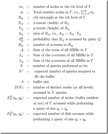
Assume the following notation:

The authors of [28, 42] assume that performance is measured by the number of nodes accessed (independent of buffering). They observe that for uniform point queries the probability of accessing Rij is just the area of Rij , namely, Aij . They point out that the level of T in which Rij resides is immaterial as all rectangles containing Q (and only those) need to be retrieved. Accordingly, for a point query, the expected number of nodes retrieved as derived in [28] is the sum of node areas∗:

which is the sum of the areas of all rectangles (both leaf level MBRs as well as MBRs of internal nodes).

We now turn our attention to region queries. Let ((a, b), (c, d)) denote an axis-parallel rectangle with bottom left and top right corners (a, b) and (c, d), respectively. Consider a rectangular query Q = (Qbl, Qtr ) of size qx ×qy . Q intersects R = ((a, b), (c, d)) if and only if Qtr (the top right corner of Q) is inside the extended rectangle R! = ((a, b), (c + qx,d + qy )), as illustrated in Figure 21.10.

Kamel and Faloutsos infer that the probability of accessing R while performing Q is the area of R!, as the region query Q is equivalent to a point query Qtr where all rectangles in T have been extended as outlined above. Thus, the expected number of nodes retrieved (as derived in [28]) is:

Equation 21.2 illustrates the fact that a good insertion/loading algorithm should cluster rectangles so as to minimize both the total area and total perimeter of the MBRs of all nodes. For point queries, on the other hand, qx = qy = 0, and minimizing the total area is enough.

In [34] the model of [28] was modified to handle query windows that fall partially outside the data space as well as data rectangles close to the boundary of the data space, as suggested by Six et al [42]. Specifically:

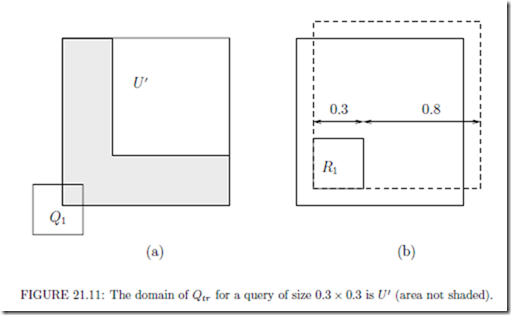
1. For uniformly distributed rectangular queries of size qx × qy the top right corner of the query region Q, cannot be an arbitrary point inside the unit square if the entire query region is to fit within the unit square. For example, if qx = qy = 0.3, a query such as Q1 in Figure 21.11a should not be allowed. Rather, Qtr must be

inside the box U ! = [qx, 1] × [qy , 1].

2. The probability of accessing a rectangle R = ((a, b), (c, d)) is not always the area of R! = ((a, b), (c + qx ,d + qy )) as this value can be bigger than one. For example, in Figure 21.11b, the probability that a query of size 0.8 × 0.8 accesses rectangle R1 should not be 1.1 · 1.1 = 1.21, which is the area of the extended rectangle R! , obtained by applying the original formula. Rather, the access probability is the percentage of U ! covered by the rectangle R! ∩ U !.

Thus, we change the probability of accessing rectangle i of level j to:

In [35] the R-tree model was expanded to take into account the distribution of the input data. Specifically, rather than being uniformly distributed, the query regions were assumed to be distributed according to the input data distribution.

The above models do not consider the impact of the buffer. In [35] a buffer model is integrated with the query model. Specifically, under uniformly distributed point queries, the probability of accessing rectangle Rij while performing a query is Aij . Accordingly, the probability that Rij is not accessed during the next N queries is P [Bij = 0|N ] = (1 − Aij )N .

Thus, P [Bij ≥ 1|N ] = 1 − (1 − Aij )N and the expected number of distinct nodes accessed in N queries is,

Note that D(0) = 0 < β and D(1) = A (which may or may not be bigger than β). The buffer, which is initially empty, first becomes full after performing N ∗ queries, where N ∗ is the smallest integer that satisfies D(N ∗) ≥ β. The value of N ∗ can be determined by a simple binary search.

While the buffer is not full the probability that Rij is in the buffer is equal to P [Bij ≥ 1].

The probability that a random query requires a disk access for Rij is Aij · P [Bij = 0].

Since the steady state buffer hit probability is approximately the same as the buffer hit probability after N ∗ queries, the expected number of disk accesses for a point query at steady state is

In [34] the authors compare the model to simulation and explore the I/O impact of pinning the top levels of an R-tree into the buffer.

Other analytical models include the following. The odoridis and Sellis [65] provide a fully analytical model that does not require the R-tree MBRs as input. In [17], a technique is developed for analyzing R-tree performance with skewed data distributions. The technique uses the concept of fractal dimension to characterize the data set and resultant R-tree performance. Analysis has also been used for estimating the performance of R-tree based spatial joins [26, 66] and nearest neighbor queries [45, 64].