Splay Trees:Analysis

Analysis

We will next like to look at the “amortized” time taken by splay operations. Amortized time is the average time taken over a worst case sequence of operations.

For the purpose of analysis, we give a positive weight w(x) to (any) item x in the tree. The weight function can be chosen completely arbitrarily (as long it is strictly positive). For analysis of splay trees we need some definitions (or nomenclature) and have to fix some parameters.

Weight of item x: For each item x, an arbitrary positive weight w(x) is associated (see Section 12.4 for some examples of function w(x)).

Size of node x: Size(x) is the sum of the individual weights of all items in the sub- tree rooted at the node x.

Rank of node x: Rank of a node x is log2(size(x)).

Potential of a tree: Let α be some positive constant (we will discuss choice of α later), then the potential of a tree T is taken to be α(Sum of rank(x) for all nodes x ∈ T ) = α ),x∈T rank(x).

Amortized Time: As always, Amortized time = Actual Time + New Potential − Old Potential.

Running Time of Splaying: Let β be some positive constant, choice of β is also discussed later but β ≤ α, then the running time for splaying is β×Number of rotations.

If there are no rotations, then we charge one unit for splaying.

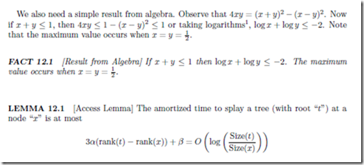
We also need a simple result from algebra. Observe that 4xy = (x + y)2 − (x − y)2. Now if x + y ≤ 1, then 4xy ≤ 1 − (x − y)2 ≤ 1 or taking logarithms1, log x + log y ≤ −2. Note

Proof We will calculate the change in potential, and hence the amortized time taken in each of the three cases.

Let s( ) denote the sizes before rotation(s) and s!( ) be the sizes after rotation(s). Let r( ) denote the ranks before rotation(s) and r!( ) be the ranks after rotation(s).

Case 1– x and parent(x) are both left (or both right) children  Please refer to Figure 12.2. Here, s(x)+ s (z) ≤ s (x), or s! (x) + s! (x) ≤ 1. Thus, by Fact 12.1,

THEOREM 12.1 Time for m accesses on a tree having at most n nodes is O((m + n) log n)

Proof Let the weight of each node x be fixed as 1/n. As there are n nodes in the entire tree, the total weight of all nodes in the tree is 1.

If t is the root of the tree then, size(t) = 1 and as each node x has at least one node (x itself) present in the subtree rooted at x (when x is a leaf, exactly one node will be present), for any node x, size(x) ≥ (1/n). Thus, we have following bounds for the ranks— r(t) ≤ 0 and r(x) ≥ − log n.

Or, from Lemma 12.1, amortized time per splay is at most 1 + 3 log n. As maximum possible value of the potential is n log n, maximum possible potential drop is also O(n log n), the theorem follows.

We will generalize the result of Theorem 12.1 in Section 12.4, where we will be choosing some other weight functions, to discuss other optimality properties of Splay trees.

Access and Update Operations

We are interested in performing following operations:

1. Access(x)— x is a key value which is to be searched.

2. Insert(x)— a node with key value x is to be inserted, if a node with this key value is not already present.

3. Delete(x)— node containing key value x is to be deleted.

4. Join(t1, t2)— t1 and t2 are two trees. We assume that all items in tree t1 have smaller key values than the key value of any item in the tree t2. The two trees are to be combined or joined into a single tree as a result, the original trees t1 and t2 get “destroyed”.

5. Split(x, t)— the tree t is split into two trees (say) t1 and t2 (the original tree is “lost”). The tree t1 should contain all nodes having key values less than (or equal to) x and tree t2 should contain all nodes having key values strictly larger than x.

We next discuss implementation of these operations, using a single primitive operation— splay. We will show that each of these operations, for splay trees can be implemented using O(1) time and with one or two “splay” operations.

Access(x, t) Search the tree t for key value x, using the routines for searching in a “binary search tree” and splay at the last node— the node containing value x, in case the search is successful, or the parent of “failure” node in case the search is unsuccessful.

Join(t1, t2) Here we assume that all items in splay tree t1 have key values which are smaller than key values of items in splay tree t2, and we are required to combine these two splay trees into a single splay tree.

Access largest item in t1, formally, by searching for “+∞”, i.e., a call to Access(+∞, t1). As a result the node containing the largest item (say r) will become the root of the tree t1. Clearly, now the root r of the splay tree t1 will not have any right child. Make the root of the splay tree t2 the right child of r, the root of t1, as a result, t2 will become the right sub-tree of the root r and r will be the root of the resulting tree.

Split(x, t) We are required to split the tree t into two trees, t1 containing all items with key values less than (or equal to) x and t2, containing items with key values greater than x.

If we carry out Access(x, t), and if a node with key value x is present, then the node containing the value x will become the root. We then remove the link from node containing the value x to its right child (say node containing value y); the resulting tree with root, containing the value x, will be t1, and the tree with root, containing the value y, will be the required tree t2.

And if the item with key value x is not present, then the search will end at a node  Splay Trees 12-7 (say) containing key value z. Again, as a result of splay, the node with value z will become the root. If z > x, then t1 will be the left subtree of the root and the tree t2 will be obtained by removing the edge between the root and its left child.

Otherwise, z < x, and t2 will be the right subtree of the root and t1 will be the resulting tree obtained by removing the edge between the root and its right child.

Insert(x, t) We are required to insert a new node with key value x in a splay tree t. We can implement insert by searching for x, the key value of the item to be inserted in tree t using the usual routine for searching in a binary search tree.

If the item containing the value x is already present, then we splay at the node containing x and return. Otherwise, assume that we reach a leaf (say) containing key y, y j= x. Then if x < y, then add the new node containing value x as a left child of node containing value y, and if x> y, then the new node containing the value x is made the right child of the node containing the value y, in either case we splay at the new node (containing the value x) and return.

Delete(x, t) We are required to delete the node containing the key value x from the splay tree t. We first access the node containing the key value x in the tree t— Access(x, t). If there is a node in the tree containing the key value x, then that node becomes the root, otherwise, after the access the root will be containing a value different from x and we return(−1)— value not found. If the root contains value x, then let t1 be the left subtree and t2 be the right subtree of the root.

Clearly, all items in t1 will have key values less than x and all items in t2 will have key values greater than x. We delete the links from roots of t1 and t2 to their parents (the root of t, the node containing the value x). Then, we join these two subtrees — Join(t1, t2) and return.

Observe that in both “Access” and “Insert”, after searching, a splay is carried out. Clearly, the time for splay will dominate the time for searching. Moreover, except for splay, everything else in “Insert” can be easily done in O(1) time. Hence the time taken for “Access” and “Insert” will be of the same order as the time for a splay. Again, in “Join”, “Split” and “Delete”, the time for “Access” will dominate, and everything else in these operations can again be done in O(1) time, hence “Join”, “Split” and “Delete” can also be implemented in same order of time as for an “Access” operation, which we just saw is, in turn, of same order as the time for a splay. Thus, each of above operations will take same order of time as for a splay. Hence, from Theorem 12.1, we have

THEOREM 12.2 Time for m update or access operations on a tree having at most n nodes is O((m + n) log n).

Observe that, at least in amortized sense, the time taken for first m operations on a tree which never has more than n nodes is the same as the time taken for balanced binary search trees like AVL trees, 2-3 trees, etc.