algorithms

Voronoi Diagrams Recall the post-office problem mentioned in the introduction. Here we want to preprocess a set S of n points, referred to as sites , in the plane such that we can answer the query: which site in S is closest to a given query point q ? In order to solve this problem we can divide the plane into regions according to the nearest-neighbor rule: each site s gets assigned the region which is closest to s . This subdivision, which compactly captures the distance information inherent in a given configuration, is called the Voronoi diagram of S —see Fig. 62.7(a). More formally, the Voronoi diagram of a set of sites S = { s 1 ,... , s n } in R d , which we refer to as Vor( S ), partitions space into n regions—one for each site—such that the region for a site s i consists of all points that are closer to s i than to any other site s j ∈ S . The set of points that are closest to a particular site s i forms the so-called Voronoi cell of s i , and is denoted by V ( s i ). Thus, w...

Convex Hulls A set A ⊂ R d is convex if for any two points p, q ∈ A the segment pq is completely contained in A . The convex hull of a set S of objects is the smallest convex set that contains all objects in S , that is, the most tightly fitting convex bounding volume for S . For example, if S is a set of objects in the plane, we can obtain the convex hull by taking a large rubber band around the objects and then releasing the band; the band will snap around the objects and the resulting shape is the convex hull. More formally, we can define C H ( S ) as the intersection of all convex sets containing all objects in S : We denote the convex hull of the objects in S by C H ( S ). It is easy to see that the convex hull of a set of line segments in the plane is the same as the convex hull of the endpoints of the segments. More generally, the convex hull of a set of bounded polygonal objects in R d is the same as the convex hull of the vertices of the objects. Therefore we will restri...

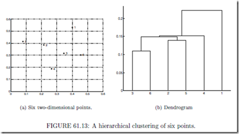
Clustering Cluster analysis [6, 7, 33, 39] groups data objects based on information found in the data that describes the objects and their relationships. The goal is that the objects in a group be similar (or related) to one another and different from (or unrelated to) the objects in other groups. The greater the similarity (or homogeneity) within a group, and the greater the difference between groups, the ‘better’ or more distinct the clustering. Hierarchical and Partitional Clustering The most commonly made distinction between clustering techniques is whether the resulting clusters are nested or unnested or, in more traditional terminology, whether a set of clusters is hie r a r chi c a l or p a rtitional . A partitional or unnested set of clusters is simply a division of the set of data objects into non-overlapping subsets (clusters) such that each data object is in exactly one subset, i.e., a partition of the data objects. The most common partitional clustering algorithm is K-m...

Data Structures for Query Processing Query evaluation is performed in main memory in several steps as outlined in Figure 60.2. Starting with the high-level input query expressed in a declarative language called SQL (see, for example, [ 2]) the Parser scans, parses, and validates the query. The goal is to check whether the query is formulated according to the syntax rules of the language supported in the DBMS. The parser also validates that all attribute and relation names are part of the database schema that is being queried. The parser produces a parse tree which serves as input to the Query Translation and R ewrite module shown underneath the parser. Here the query is translated into an internal representation, which is based on the relational algebra notation [1]. Besides its compact form, a major advantage of using relational algebra is that there exist transformations (re- write rules) between equivalent expressions to explore alternate, more efficient forms of the same qu...

Space Filling Curves: Order in Many Dimensions As explained above, our interest in space filling curves (SFCs) comes from two sources. The first one is the fact that we aim at exploiting the typical database support mechanisms that a conventional database management system (DBMS) offers, such as support for transactions and recovery. On the data structures level, this support is automatic if we resort to a data structure that is inherently supported by a DBMS. These days, this is the case for a number of one dimensional data structures, such as those of the B-tree family (see Chapter 15). In addition, spatial database management systems support one of a small number of multidimensional data structures, such as those of the R-tree family (see Chapter 21) or of a grid based structure. The second reason for our interest in space filling curves is the general curiosity in the gap between one dimension and many: In what way and to what degree can we bridge this gap for the sake of supporting ...