The Web as a Dynamic Graph:Properties of Web Graphs and Web Algorithmics and Conclusions

Properties of Web Graphs and Web Algorithmics

The properties of web graphs that have been studied analytically are average shortest path lengths between two vertices, size of giant components and their distributions. All these properties have been studied extensively for Gn,p class of random graphs. Seminal work in this area for graphs whose degrees were given was done by Malloy and Reed [23] who came up with a precise condition under which phase transition would take place and giant components as large as the graph itself would start to show up. In what follows we will discuss these issues using generating functions as done by Newman, Strogatz, and Watts [28] primarily because of the simplicity with which these reasonably complex issues can be handled in an integrated framework.

Generating Function Framework

Following [28] we define for a large undirected graph with N nodes the generating function

where pk is the probability that a randomly chosen vertex has degree k. We assume that the probability distribution is correctly normalised, i.e. G0(1) = 1. G0(x) can also represent graphs where we know the exact number nk of vertices of degree k by defining

The denominator is required to ensure that the generating function is properly normalised. Consider the function [G0(x)]2 . Note that coefficient of the power of xn in [G0(x)]2 is given i+j=n pipj which is nothing but the probability of choosing two vertices such that the sum of their degrees is n. The product of two or more generating functions representing different degree distributions can be interpreted in the same way to represent probability distributions reflecting independent choices from the two or more distributions involved.

Consider the problem of estimating the average degree of a vertex chosen at random. The average degree is given by k kpk which is also equal to Gl (1). Interestingly the average degree of a vertex chosen at random and the average degree of a vertex pointed to by a random edge are different. A random edge will point to a vertex with probability proportional to the degree of the vertex which is of the order of kpk. The appropriately normalised distribution is given by the generating function

The generating function given above in eq. (51.8) will have to be divided by x if we wanted to consider the distribution of degree of immediate neighbors excluding the edges by which one reached them. We will denote that generating function by G1(x). The neighbors of these immediate neighbors are the second neighbors of the original node. The probability that any of the second neighbors connect to any of the immediate neighbors or one another is no more than order of N −1 and hence can be neglected when N is large. Under this assumption the distribution of the second neighbors of the originally randomly chosen node is

Average Path Length

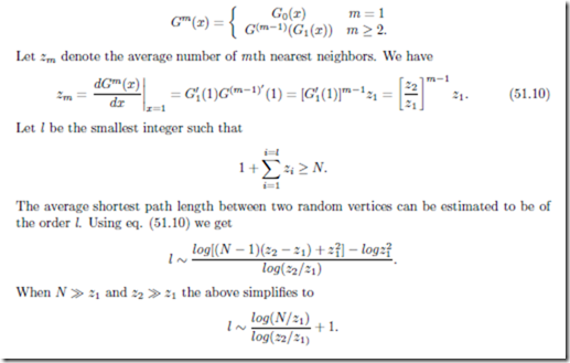
We can extend this reasoning to estimate the distributions for the mth neighbors of a randomly chosen node. The generating function for the distribution for the mth neighbor, denoted by Gm(x), is given by

There do exist more rigorous proofs of this result for special classes of random graphs. The most interesting observation made in [28] is that only estimates of nearest and second nearest neighbors are necessary for calculation of average shortest path length, and that making these purely local measurements one can get a fairly good measure of the average shortest distance which is a global property. One, of course, is assuming that the graph is connected or one is limiting the calculation to the giant connected component.

Emergence of Giant Components

Consider the process of choosing a random edge and determining the component(s) of which one of its end nodes is a part. If there are no other edges incident at that node then that node is a component by itself. Otherwise the end node could be connected to one component, or two components and so on. Therefore, the probability of a component attached to the end of a random edge is the sum of the probability of the end node by itself, the end node connected to one other component, or two other components and so on. If H1(x) is the generating function for the distribution of the sizes of the components which are attached to one of the ends of the edge, then H1(x) satisfies the recursive equation

H1(x) = xG1(H1(x)).                            (51.11)

Note that each such component is associated with the end of an edge. Therefore, the com- ponent associated with a random vertex is a collection of such components associated with the ends of the edges leaving the vertex, and so, H0(x) the generating function associated with size of the whole component is given by

This condition is the same as that obtained by Molloy and Reed in [23]. The sum on the l.h.s. of eq. (51.16) increases monotonically as edges are added to the graph. Therefore, the giant component comes into existence when the sum on the l.h.s. of eq. (51.16) becomes positive. Newman et al. state in [28] that once there is a giant component in the graph, then H0(x) generates the probability distribution of the sizes of the components excluding the giant component. Molloy and Reed have shown in [24] that the giant component almost surely has cN + o(N ) nodes. It should be remembered that the results in [23, 24, 28] are all for graphs with specified degree sequences. As such they are applicable to graphs with power law degree distributions. However, web graphs are directed and a model that explains adequately the structure consistent with all that is known experimentally is still to be developed.

Search on Web Graphs

Perhaps the most important algorithmic problem on the Web is mining of data. We will, however, have not much to say about it partly because it has been addressed in Chapter 50, but also because we want to focus on issues that become specially relevant in an evolving web graph. Consider the problem of finding a path between two nodes in a graph. On the Web this forms the core of the peer to peer (P2P) search problem defined in the context of locating a particular file on the Web when there is no information available in a global directory about the node on which the file resides. The basic operation available is to pass messages to neighbors in a totally decentralised manner. Normally a distributed message passing flooding technique on an arbitrary random network would be suspect suspect because of the very large number of messages that may be so generated. Under the assumption that a node knows about the identities of its neighbors and perhaps neighbors’ neighbors, Adamic et al. [1] claim, experimentally through simulations, that in power law graphs with N nodes the average search time is of the order of N 0.79 (graphs are undirected and power law coefficients for the generated graphs is 2.1) when the search is totally random. The intuitive explanation is that even in a random search the search process tends to gravitate towards nodes of high degree. When the strategy is to choose to move to the highest degree neighbor the exponent comes down to 0.70. Adamic et al. [1] have come up a with a fairly simple analysis to explain why random as well as degree directed search algorithms need not have time complexity more than rootic in N (reported exponent is 0.1). In what follows we develop the argument along the lines done by Mehta [26] whose analysis, done assuming that the richest node is selected on the basis of looking at the neighbors and neighbors’ neighbors, has resulted in a much sharper bound than the one in [1]. We will assume that the cut off degree, m, beyond which the the probability distribution is small enough to be ignored is given by m = N 1/α [3].

Using

The search proceeds by choosing at each step the highest degree node among the n neighbors of the current node. The total time taken can be estimated to be the sum of the number of nodes traversed at each step. The number of steps itself can be bounded by noting that the sum of the number of steps at each step can not exceed the size of the graph. Let pmax(x, n) be the distribution of the degree of the richest node (largest degree node) among the n neighbors of a node. Determining the richest node is equivalent to taking the maximum of n independent random variables and in terms of the CDF P (x),

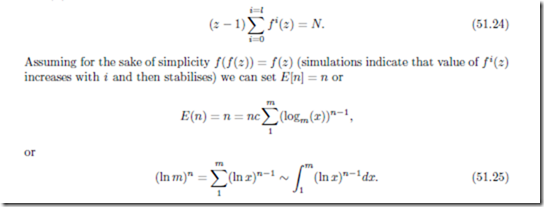
Note that if the number of neighbors of every node on the average is z, then the number of second neighbors seen when one is at the current richest node is f (z)(z − 1). this is because one of the neighbors of every other node is the richest node. At the next step, the expected degree of the node whose current degree is f (z) is given by E(f (z)) = f (f (z)) and the number of second neighbors seen at this stage correspondingly is f (f (z))(z − 1).

The overlap between two successive computations of neighbors takes place only when there is an edge which makes a node a neighbor as well as the second neighbor. However, the probability of this happening is of the order of N −1 and can be ignored in the limit for large N. Therefore we can assume that at every stage new nodes are scanned and the number of steps, l, is controlled by

Taking α to be 2.1 the number of steps would be of the order of N 0.52/ ln m. Mehta [26] also reports results of simulations carried out on graphs generated with α equal to 2.1 using the method given in [3]. The simulations were carried out on the giant components. He reports the number of steps to be growing proportional to N 0.34. The simulation results are very preliminary as the giant components were not very large (largest was of the order of 20 thousand nodes).

Crawling and Trawling

Crawling can be looked upon as a process where an agent moves along the nodes and edges of a randomly evolving graph. Off-line versions of the Web which are the basis of much of what is known experimentally about the Web have been obtained essentially through this process. Cooper and Frieze [14] have attempted to study the expected performance of a crawl process where the agent makes a fixed number of moves between the two successive time steps involving addition of nodes and edges to the graph. The results are fairly pessimistic. Expected proportion of unvisited nodes is of order of 0.57 of the graph size when the edges are added uniformly at random. The situation is even worse when the edges are distributed in proportion to the degree of nodes. The proportion of the unvisited vertices increases to 0.59.

Trawling, on the other hand, involves analyzing the web graph obtained through a crawl for subgraphs which satisfy some particular structure. Since the web graph representation may run into Tera bytes of data, the traditional random access model for computing the algorithmic complexity looses relevance. Even the standard external memory models may not apply as data may be on tapes and may not fit totally on the disks available. In these environments it may even be of interest to develop algorithms where the figure of merit may be the number of passes made over the graph represented on tape [29]. In any case the issue in trawling is to design algorithms that efficiently stream data between secondary and main memory.

Kumar et al. discuss in [22] the design of trawling algorithms to determine bipartite cores in web graphs. We will focus only on the core issue here which is that the size of the web graph is huge in comparison to the cores that are to be detected. This requires pruning of the web graph before algorithms for core detection are run. If (i, j) cores (i represents outdegree and j indegree) have to be detected then all nodes with outdegree less than i and indegree less than j have to be pruned out. This can be done with repeated sorting of the web graph by in and out degrees and keeping track of only those nodes that satisfy the pruning criteria. If an index is kept in memory of all the pruned in vertices then repeated sorting may also be avoided.

The other pruning strategy discussed in [22] is the so called inclusion exclusion pruning in which the focus at every step is to either discover an (i, j) core or exclude a node from further contention. Consider a node x with outdegree equal to i (these will be termed fans) and let Γ(x) be the set of nodes that are potentially those with which x could form an (i, j) core (called centers). An (i, j) core will be formed if and only if there are i − 1 other nodes all pointing to each node in Γ(x). While this condition is easy to check if there are two indices in memory, the whole process can be done in two passes. In the first identify all the fans with out degree i. Output for each such fan the set of i centers adjacent to it. In the second pass use an index on the destination id to generate the set of fans pointing to each of the i centers and compute the intersection of these sets. Kumar et al. [22] mention that this process can be batched with index only being maintained of the centers that result out of the fan pruning process. If we maintain the set of fans corresponding to the centers that have been indexed, then using the dual condition that x is a part of the core if and only if the intersection of the sets Γ−1(x) has size at least j. If this process results in identification of a core then a core is outputted other wise the node x is pruned out. Kumar et al. [22] claim that this process does not result in any not yet identified cores to be eliminated.

The area of trawling is in its infancy and techniques that will be developed will depend primarily on the structural properties being discovered. It is likely to be influenced by the underlying web model and the whether any semantic information is also used in defining the structure. This semantic information may be inferred by structural analysis or may be available in some other way. Development of future web models will depend largely on our understanding of the web, and they themselves will influence the algorithmic techniques developed.

Conclusions

The modeling and analysis of web as a dynamic graph is very much in its infancy. Continuous mathematical models, which has been the focus of this write up provides good intuitive understanding at the expense of rigour. Discrete combinatorial models that do not brush the problems of proving concentration bounds under the rug are available for very simple growth models. These growth models do not incorporate death processes, or the issues relating to aging (newly created pages are more likely to be involved in link gen- eration processes) or for that matter that in and out degree distributions on the web are not independent and may depend upon the underlying community structure. The process of crawling which can visit only those vertices that have at least one edge pointing to it gives a very limited understanding of degree distributions. There are reasons to believe that a significantly large number of pages on the web have only out hyperlinks. All this calls for extensive experimental investigations and development of mathematical models that are tractable and help both in development of new analytical as well as algorithmic techniques. The author would like to acknowledge Amit Agarwal who provided a willing sounding board and whose insights have significantly influenced the author’s approach on these issues.