Elimination Structures in Scientific Computing:The Elimination Tree
The Elimination Tree
Gaussian elimination of a symmetric positive definite matrix A, which factors the matrix A into the product of a lower triangular matrix L and its transpose LT , A = LLT , is one of the fundamental algorithms in scientific computing. It is also known as Cholesky factorization. We begin by considering the graph model of this computation performed on a symmetric matrix A that is sparse, i.e., few of its matrix elements are nonzero. The number of nonzeros in L and the work needed to compute L depend strongly on the (symmetric) ordering of the rows and columns of A. The graph model of sparse Gaussian elimination was introduced by Parter [58], and has been called the elimination game by Tarjan [70]. The goal of the elimination game is to symmetrically order the rows and columns of A to minimize the number of nonzeros in the factor L.
We consider a sparse, symmetric positive definite matrix A with n rows and n columns, and its adjacency graph G(A) = (V, E) on n vertices. Each vertex in v ∈ V corresponds to the v-th row of A (and by symmetry, the v-th column); an edge (v, w) ∈ E corresponds to the nonzero avw (and by symmetry, the nonzero awv ). Since A is positive definite, its diagonal elements are positive; however, by convention, we do not explicitly represent a diagonal element avv by a loop (v, v) in the graph G(A). (We use v, w, ... to indicate unnumbered vertices, and i, j, k, ... to indicate numbered vertices in a graph.)
We view the vertices of the graph G(A) as being initially unnumbered, and number them from 1 to n, as a consequence of the elimination game. To number a vertex v with the next available number, add new fill edges to the current graph to make all currently unnumbered neighbors of v pairwise adjacent. (Note that the vertex v itself does not acquire any new neighbors in this step, and that v plays no further role in generating fill edges in future numbering steps.)
The graph that results at the end of the elimination game, which includes both the edges in the edge set E of the initial graph G(A) and the set of fill edges, F , is called the filled graph. We denote it by G+ (A) = (V, E ∪ F ). The numbering of the vertices is called an elimination ordering, and corresponds to the order in which the columns are factored.
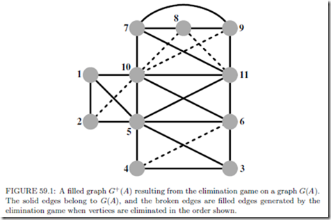
An example of a filled graph resulting from the elimination game on a graph is shown in Fig. 59.1. We will use this graph to illustrate various concepts throughout this paper.
The goal of the elimination game is to number the vertices to minimize the fill since it would reduce the storage needed to perform the factorization, and also controls the work in the factorization. Unfortunately, this is an NP-hard problem [74]. However, for
classes of graphs that have small separators, it is possible to establish upper bounds on the number of edges in the filled graph, when the graph is ordered by a nested dissection algorithm that recursively computes separators. Planar graphs, graphs of ‘well-shaped’ finite element meshes (aspect ratios bounded away from small values), and overlap graphs possess elimination orderings with bounded fill. Conversely, the fill is large for graphs that do not have good separators.
Approximation algorithms that incur fill within a polylog factor of the optimum fill have been designed by Agrawal, Klein and Ravi [1]; but since it involves finding approximate concurrent flows with uniform capacities, it is an impractical approach for large problems. A more recent approximation algorithm, due to Natanzon, Shamir and Sharan [57], limits fill to within the square of the optimal value; this approximation ratio is better than that of the former algorithm only for dense graphs.
The elimination game produces sets of cliques in the graph. Let hadj+(v) (ladj+(v)) denote the higher-numbered (lower-numbered) neighbors of a vertex v in the graph G+ (A); in the elimination game, hadj+(v) is the set of unnumbered neighbors of v immediately prior to the step in which v is numbered. When a vertex v is numbered, the set {v}∪hadj+(v) becomes a clique by the rules of the elimination game. Future numbering steps and consequent fill edges added do not change the adjacency set (in the filled graph) of the vertex v. (We will use hadj(v) and ladj(v) to refer to higher and lower adjacency sets of a vertex v in the original graph G(A).)
The Elimination Tree Data Structure
We define a forest from the filled graph by defining the parent of a vertex v to be the lowest numbered vertex in hadj+(v). It is clear that this definition of parent yields a forest since the parent of each vertex is numbered higher than itself. If the initial graph G(A) is
connected, then indeed we have a tree, the elimination tree; if not we have an elimination forest.
In terms of the Cholesky factor L, the elimination tree is obtained by looking down each column below the diagonal element, and choosing the row index of the first subdiagonal nonzero to be the parent of a column. It will turn out that we can compute the elimination tree corresponding to a matrix and a given ordering without first computing the filled graph or the Cholesky factor.
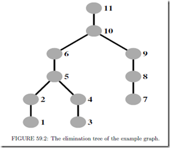
The elimination tree of the graph in Fig. 59.1 with the elimination ordering given there is shown in Fig. 59.2.
A fill path joining vertices i and j is a path in the original graph G(A) between vertices i and j, all of whose interior vertices are numbered lower than both i and j. The following theorem offers a static characterization of what causes fill in the elimination game.
THEOREM 59.1 [64] The edge (i, j) is an edge in the filled graph if and only if a fill path joins the vertices i and j in the original graph G(A).
In the example graph in Fig. 59.1, vertices 9 and 10 are joined a fill path consisting of the interior vertices 7 and 8; thus (9, 10) is a fill edge. The next theorem shows that an edge in the filled graph represents a dependence relation between its end points.
THEOREM 59.2 [69] If (i, j) is an edge in the filled graph and i < j, then j is an ancestor of the vertex i in the elimination tree T (A).
This theorem suggests that the elimination tree represents the information flow in the elimination game (and hence sparse symmetric Gaussian elimination). Each vertex i influences only its higher numbered neighbors (the numerical values in the column i affect only those columns in hadj+(i)). The elimination tree represents the information flow in a minimal way in that we need consider only how the information flows from i to its parent in the elimination tree. If j is the parent of i and R is another higher neighbor of i, then since the higher neighbors of i form a clique, we have an edge (j, R) that joins j and R; since by Theorem 59.2, R is an ancestor of j, the information from i that affects R can be viewed as being passed from i first to j, and then indirectly from j through its ancestors on the path in the elimination tree to R.
An immediate consequence of the Theorem 59.2 is the following result.
COROLLARY 59.1 If vertices i and j belong to vertex-disjoint subtrees of the elimination tree, then no edge can join i and j in the filled graph.
Viewing the dependence relationships in sparse Cholesky factorization by means of the elimination tree, we see that any topological reordering of the elimination tree would be an elimination ordering with the same fill, since it would not violate the dependence relation- ships. Such reorderings would not change the fill or arithmetic operations needed in the factorization, but would change the schedule of operations in the factorization (i.e., when a specific operation is performed). This observation has been used in sparse matrix factorizations to schedule the computations for optimal performance on various computational platforms: multiprocessors, hierarchical memory machines, external memory algorithms, etc. A postordering of the elimination tree is typically used to improve the spatial and temporal data locality, and thereby the cache performance of sparse matrix factorizations.
There are two other perspectives from which we can view the elimination tree.
Consider directing each edge of the filled graph from its lower numbered endpoint to its higher numbered endpoint to obtain a directed acyclic graph (DAG). Now form the transitive reduction of the directed filled graph; i.e., delete an edge (i, k) whenever there is a directed path from i to k that does not use the edge (i, k) (this path necessarily consists of at least two edges since we do not admit multiple edges in the elimination game). The minimal graph that remains when all such edges have been deleted is unique, and is the elimination tree.
One could also obtain the elimination tree by performing a depth-first search (DFS) in the filled graph with the vertex numbered n as the initial vertex for the DFS, and choosing the highest numbered vertex in ladj+(i) as the next vertex to search from a vertex i.
An Algorithm
We begin with a consequence of the repeated application of the following fact: If a vertex i is adjacent to a higher numbered neighbor k in the filled graph, and k is not the parent of i, pi, in the elimination tree, then i is adjacent to both k and pi in the filled graph; when i is eliminated, by the rules of the elimination game, a fill edge joins pi and k.
THEOREM 59.3 If (i, k) is an edge in the filled graph and i < k, then for every vertex j on an elimination tree path from i to k, (j, k) is also an edge in the filled graph.
This theorem leads to a characterization of ladj+(k), the set of lower numbered neighbors of a vertex k in the filled graph, which will be useful in designing an efficient algorithm for computing the elimination tree. The set ladj+(k) corresponds to the column indices of nonzeros in the k-th row of the Cholesky factor L, and ladj(k) corresponds to the column indices of nonzeros in the lower triangle of the k-th row of the initial matrix A.
THEOREM 59.4 [51] Every vertex in the set ladj+(k) is a vertex reachable by paths in the elimination tree from a set of leaves to k; each leaf l corresponds to a vertex in the set ladj(k) such that no proper descendant d of l in the elimination tree belongs to the set ladj(k).
Theorem 59.4 characterizes the k-th row of the Cholesky factor L as a row subtree Tr (k)
FIGURE 59.3: An algorithm for computing an elimination tree. Initially each vertex is in a subtree with it as the root.
of the elimination subtree rooted at the vertex k, and pruned at each leaf l. The leaves of the pruned subtree are contained among ladj(k), the column indices of the nonzeros in (the lower triangle of) the k-th row of A.
In the elimination tree in Fig. 59.2, the pruned elimination subtree corresponding to row 11 has two leaves, vertices 5 and 7; it includes all vertices on the etree path from these leaves to the vertex 11.
The observation above leads to an algorithm, shown in Fig. 59.3, for computing the elimination tree from the row structures of A, due to Liu [51].
This algorithm can be implemented efficiently using the union-find data structure for disjoint sets. A height compressed version of the p. array, ancestor, makes it possible to compute the root fast; and union by rank in merging subtrees helps to keep the merged tree shallow. The time complexity of the algorithm is O(eα(e, n) + n), where n is the number of vertices and e is the number of edges in G(A), and α(e, n) is a functional inverse of Ackermann’s function. Liu [54] shows experimentally that path compression alone is more efficient than path compression and union by rank, although the asymptotic complexity of the former is higher. Zmijewski and Gilbert [75] have designed a parallel algorithm for computing the elimination tree on distributed memory multiprocessors.
The concept of the elimination tree was implicit in many papers before it was formally identified. The term elimination tree was first used by Duff [17], although he studied a slightly different data structure; Schreiber [69] first formally defined the elimination tree, and its properties were established and used in several articles by Liu. Liu [54] also wrote an influential survey that delineated its importance in sparse matrix computations; we refer the reader to this survey for a more detailed discussion of the elimination tree current as of 1990.
A Skeleton Graph
The filled graph represents a supergraph of the initial graph G(A), and a skeleton graph represents a subgraph of the latter. Many sparse matrix algorithms can be made more efficient by implicitly identifying the edges of a skeleton graph G−(A) from the graph G(A) and an elimination ordering, and performing computations only on these edges. A skeleton graph includes only the edges that correspond to the leaves in each row subtree in Theorem 59.4. The other edges in the initial graph G(A) can be discarded, since they will be generated as fill edges during the elimination game. Since each leaf of a row subtree corresponds to an edge in G(A), the skeleton graph G−(A) is indeed a subgraph of the former. The skeleton graph of the example graph is shown in Fig. 59.4.
The leaves in a row subtree can be identified from the set ladj(j) when the elimination tree is numbered in a postordering. The subtree T (i) is the subtree of the elimination tree
Supernodes
A supernode is a subset of vertices S of the filled graph that form a clique and have the same higher neighbors outside S. Supernodes play an important role in numerical algorithms since loops corresponding to columns in a supernode can be blocked to obtain high performance on modern computer architectures. We now proceed to define a supernode formally.
A maximal clique in a graph is a set of vertices that induces a complete subgraph, but adding any other vertex to the set does not induce a complete subgraph. A supernode is a maximal clique {is, is+1,... , is+t−1} in a filled graph G (A) such that for each 1 ≤ j ≤ t−1,
Let hd+(is) ≡ |hadj+(is)|; since hadj+ (is) ⊆ {is+1,... , is+j }∪ hadj+(is+j ), the relationship between the higher adjacency sets can be replaced by the equivalent test on higher degrees: hd+(is) = hd+(is+j ) + j.
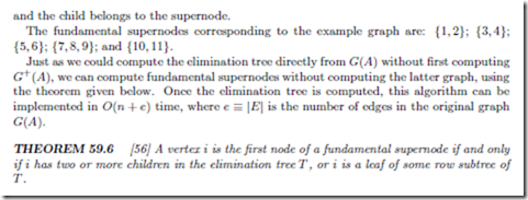
In practice, fundamental supernodes, rather than the maximal supernodes defined above, are used, since the former are easier to work with in the numerical factorization. A fundamental supernode is a clique but not necessarily a maximal clique, and satisfies two additional conditions: (1) is+j−1 is the only child of the vertex is+j in the elimination tree, for each 1 ≤ j ≤ t − 1; (2) the vertices in a supernode are ordered consecutively, usually by post-ordering the elimination tree. Thus vertices in a fundamental supernode form a path in the elimination tree; each of the non-terminal vertices in this path has only one child,


Comments
Post a Comment