Computer Graphics:Data Structures

Data Structures

Vertices, Edges, and Faces

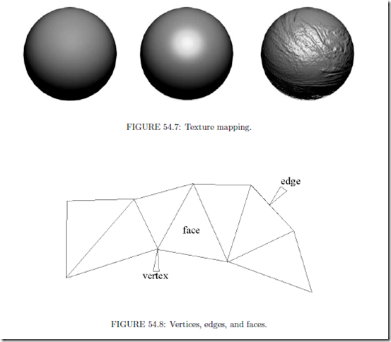
As mentioned previously, vertices, edges, and faces form the most basic elements of all polygonal representations in computer graphics. The simplest point can be represented in Cartesian coordinates in two (2D) and three dimensions (3D) as (x,y) and (x,y,z) respectively (Figure 54.8).

As a simple data structure, each vertex may then be stored as a two or three-dimensional array. Edges may then be represented by two-dimensional arrays containing the indexes of two points. Further, a face may be dimensioned based on the number of desired sides per face, and contain the indices of those edges. At first, this approach may seem acceptable, and in basic applications it is common to model each vertex, edge, and face as a separate class. Relative relationships between classes are then governed by the software to build meshes. However, modeling objects in this manner does have disadvantages.

Firstly, important information becomes difficult to track, such as the normal at each vertex, adjacency of faces, and other properties required for blending and achieving realism. Furthermore, the number of intersecting edges at each vertex may vary throughout the model, and mesh sizes between objects may be unpredictable. The ability to manage this approach then becomes increasingly difficult, with the potential for unnecessary overhead and housekeeping of relationships within the model. It then becomes necessary to create higher level data structures that go beyond these basic elements, and provide the elements necessary for efficient graphics applications.

Vertex, Normal, and Face Lists

In this storage method, list structures are used to store three, inter-dependent lists of data. The first list defines the vertexes contained in the scene as follows. Each vertex is assigned an index, and a coordinate location, or (x,y,z) point. The second list defines the normals for each vertex. Again, each normal is assigned a numbered index and a 3-D coordinate point. The final list serves to integrate the first two. Each face is identified by a numbered index, an array of vertex indexes, and an array of indexed normals for each vertex. Figure 54.9 illustrates typical examples of a similar application with vertex, face, and edge lists.

FIGURE 54.9: Example of vertex, normal, and face lists.

In the table, three specific lists are evident. The first list represents each vertex in the model as it is defined in 3D space. The “vertex” column defines the id, index, or label of the vertex. The x, y, and z coordinates are then defined in the adjacent columns.

In the second list, six faces are defined. Each face has a label or index similar to the vertex list. However, rather than specifying coordinates in space, the adjacent column stores the id’s of the vertexes that enclose the face. Note that each face consists of four vertices, indicating that the each face will be defined by a quadrilateral.

The final list defines edges. Again, each edge definition contains a label or index column, followed by two adjacent vertex columns. The vertices of each edge define the start point and end point of each edge. In many applications of graphics, it is important to define the direction of an edge. In right handed coordinate systems, the direction of an edge will determine the direction of the normal vector which is orthogonal to the face surrounded by the edges.

Winged Edge

Although one of the oldest data structures relating to polygonal structures, the Winged Edge approach is very effective, and still widely used [5]. This structure is different from the wireframe model in that edges are the primary focal point of organization.

In the structure, each edge is stored in an indexed array, with its vertices, adjacent faces, previous, and successive edges. This allows the critical information for each edge to be stored in an array of eight integer indexes; it is both consistent and scalable between applications. The structure is

An important aspect of the Winged Edge structure is the order in which entries are listed. The edge itself has a direction, from the start vertex to the end vertex. The other entries are then defined by their proximity to the edge. If the direction of the edge were reversed, the right and left faces would change accordingly, as would the previous and succeeding entries of both the left and right traverse.

There is a time/space trade-off in using this model. What is saved in storage space adds to the needed time to find previous and successive edges. See Chapter 17 for more details.

Tiled, Multidimensional Array

In this section we will discuss a data structure that is important to most geometric implementations. In many ways, the tiled array behaves identically to matrix data structures. For instance, a p by q matrix is normally stored as a single dimension array. However, since the matrix has p-rows and q-columns, the array needs to be addressed by creating an “offset” of size q in order to traverse each row. The following example should illustrate this concept.

This represents where a 3x3 matrix is stored as an array with (3)(3) = 9 entries. In order to find the entry at row(i) = 3 and column(j) = 2 we employ the following method on the array:

We use a similar method for tiling a single bitmap into several smaller images. This is analogous to each number entry in the above array being replaced by a bitmap with n by n pixels.

“Utilizing cache hierarchy is a crucial task in designing algorithms for modern architectures.”[2] In other words, tiling is a crucial step to ensuring multi-dimensional arrays are stored in an efficient, useful manner. Indexing mechanisms are used to locate data in each dimension. For example, a p by q array is stored in a one-dimensional array of length p*q, and indexed in row-column fashion as above.

When we wish to tile a p by q matrix into n by n tiles, the number of blocks in x is defined by q/n and the number of blocks in y is defined by p/n. Therefore, to find the “tile index” or the row and column of the tile for a value (x,y) we first calculate the tile location, or bitmap within the matrix of bitmaps. Then once the bitmap is located, the pixel location within that bitmap tile is found (sub-indexed). The entire two-step process can be simplified into a single equation that is executed once. Figure 54.12 illustrates this concept.

When dealing with matrices and combining multiple bitmaps and/or data into a Tile Multidimensional Array, performance and speed can both improve substantially.

Linear Interpolation and Bezier Curves

This section will introduce one of the most significant contributions to design and graphics: the interpolated curve structure.

Linear interpolation refers to the parameterization of a straight line as a function of t, or:

L(t) = (1 − t)a + tb

where a, b are points in space. This equation represents both an affine invariant and barycentric combination of the points a and b. Affine invariance means that the point L(t) will always be collinear with the straight line through the point set {a, b}, regardless of the positioning of a and b. Describing this set as barycentric simply means that for t values between 0 and 1, L(t) will always occur between a and b. Another accurate description is that the equation L(t) is a linear “mapping” of t into some arbitrary region of space. Figure 54.13 illustrates this concept.

FIGURE 54.13: Linear interpolation.

Linear interpolation is an extremely powerful concept. It is not only the foundation of many curve approximation algorithms, but the method is also used in many non-geometric applications as well, including calculating individual pixel intensities in the Phong shading method mentioned previously.

The basic Bezier curve derivation is based on an expanded form of linear interpolation. This concept uses the parameterization of t to represent two connected lines. The curve is then derived by performing a linear interpolation between the points interpolated on each line; a sort of linear interpolation in n parts, where n is the number of control points. The following example should illustrate:

Given are three points in space, {a, b, c}. These three points form the two line segments ab and bc (Figure 54.14).

FIGURE 54.14: Expanded form of linear interpolation.

During the first “iteration” of the Bezier curve derivation, linear interpolation is per- formed on each line segment for a given t value. These points are then connected by an additional line segment. The resulting equations (illustrated in Figure 54.15) are:

This final point z, after three linear interpolations, is on the curve. Following this 3-step process for several “stepped” values for t between 0 and 1 would result in a smooth curve of z-values from a to c, and is illustrated in Figure 54.17:

This is a quadratic Bezier curve, and is represented mathematically by a linear interpolation between each set of x and y points, which were also derived through linear interpolation, for every t. By substituting the equations for x and y into the basic form, we obtain:

The “string art” algorithm described previously is also referred to as the de Causteljau algorithm. Programmatically, the algorithm performs an n-step process for each value of t, where n is the number of “control points” in the curve. In this example, {a, b, c} are the control points of the curve.

Because of their ease of implementation and versatility, Bezier curves are invaluable in CAD, CAM, and graphic design. Also, Bezier curves require only a small number of control points for an accurate definition, so the data structure is ideal for compact storage. As mentioned previously, the Bezier form is the foundation for the Postscript font definition structure.

However, the Bezier form has limitations. When several attached curves are required in a design component, it takes considerable effort, or pre-calculation, to ensure the connected curves are “fair” or continuous with each other. Merely joining the end points of the curves may not be enough, resulting in “kinks” and other undesirable effects. For this reason, the B-spline curve provides an alternative to the Bezier where continuity is important. In fact, B-spline curves have often been referred to as a “user interface” for the Bezier form.

The goal of this section was to illustrate the versatility of linear interpolation and basic iteration structures in graphics and design. If more information is desired, numerous texts are currently available which describe the properties, mathematics, and applications of Bezier and B-spline curves, including the references listed at the end of this chapter.