Data Mining:Clustering and Conclusion

Clustering

Cluster analysis [6, 7, 33, 39] groups data objects based on information found in the data that describes the objects and their relationships. The goal is that the objects in a group be similar (or related) to one another and different from (or unrelated to) the objects in other groups. The greater the similarity (or homogeneity) within a group, and the greater the difference between groups, the ‘better’ or more distinct the clustering.

Hierarchical and Partitional Clustering

The most commonly made distinction between clustering techniques is whether the resulting clusters are nested or unnested or, in more traditional terminology, whether a set of clusters is hierarchical or partitional. A partitional or unnested set of clusters is simply a division of the set of data objects into non-overlapping subsets (clusters) such that each data object is in exactly one subset, i.e., a partition of the data objects. The most common partitional clustering algorithm is K-means, whose operation is described by the psuedo-code in Figure 61.11. (K is a user specified parameter, i.e., the number of clusters desired, and a centroid is typically the mean or median of the points in a cluster.)

1: Initialization: Select K points as the initial centroids.

2: repeat

3: Form K clusters by assigning all points to the closest centroid.

4: Recompute the centroid of each cluster.

5: until The centroids do not change

FIGURE 61.11: Basic K-means algorithm.

A hierarchical or nested clustering is a set of nested clusters organized as a hierarchical tree, where the leaves of the tree are singleton clusters of individual data objects, and where the cluster associated with each interior node of the tree is the union of the clusters associated with its child nodes. Typically, hierarchical clustering proceeds in an agglomerative manner, i.e., starting with each point as a cluster, we repeatedly merge the closest clusters, until only one cluster remains. A wide variety of methods can be used to define the distance between two clusters, but this distance is typically defined in terms of the distances between pairs of points in different clusters. For instance, the distance between clusters may be the minimum distance between any pair of points, the maximum distance, or the average dis- tance. The algorithm for agglomerative clustering is described by the psuedo-code in Figure 61.12.

1: Compute the pairwise distance matrix.

2: repeat

3: Merge the closest two clusters.

4: Update the distance matrix to reflect the distance between the new cluster and the original clusters.

5: until Only one cluster remains

FIGURE 61.12: Basic agglomerative hierarchical clustering algorithm

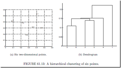
The tree that represents a hierarchical clustering is called a dendrogram, a term that comes from biological taxonomy. Figure 61.13 shows six points and the hierarchical clustering that is produced by the MIN clustering technique. This approach creates a hierarchical clustering by starting with the individual points as clusters, and then successively merges pairs of clusters with the minimum distance, i.e., that have the closest pair of points.

Nearest Neighbor Search and Multi-Dimensional Access Methods

In both the K-means and agglomerative hierarchical clustering algorithms, the time required is heavily dependent on the amount of time that it takes to find the the distance between sets of points—step 3 in both algorithms. This is true of most other clustering schemes as well, and thus, efficient implementations of clustering techniques often require considerations of nearest-neighbor search and the related area of multi-dimensional access methods. In the remainder of this section, we discuss these areas and their relevance to cluster analysis.

We begin by considering a general situation. Given a set of objects or data points, including possibly complicated data such as images, text strings, DNA sequences, polygons, etc., two issues are key to efficiently utilizing this data:

1. How can items be located efficiently? While a ‘representative’ feature vector is commonly used to ‘index’ these objects, these data points will normally be very sparse in the space, and thus, it is not feasible to use an array to store the data. Also, many sets of data do not have any features that constitute a ‘key’ that would allow the data to be accessed using standard and efficient database techniques.

2. How can similarity queries be efficiently conducted? Many applications, including clustering, require the nearest neighbor (or the k nearest neighbors) of a point. For instance, the clustering techniques DBSCAN [24] and Chameleon [37] will have a time complexity of O(n2) unless they can utilize data structures and algorithms that allow the nearest neighbors of a point to be located efficiently. As a non-clustering example of an application of similarity queries, a user may want to find all the pictures similar to a particular photograph in a database of photographs.

Techniques for nearest-neighbor search are often discussed in papers describing multi- dimensional access methods or spatial access methods, although strictly speaking the topic of multi-dimensional access methods is broader than nearest-neighbor search since it ad- dresses all of the many different types of queries and operations that a user might want to perform on multi-dimensional data. A large amount of work has been done in the area of nearest neighbor search and multi-dimensional access methods. Examples of such work include the kdb tree [14, 48], the R [28] tree, the R* tree [8], the SS-tree [34], the SR-tree [38], the X-tree [11], the GNAT tree [13], the M-tree [16], the TV tree [41], the hB tree [42], the “pyramid technique” [10], and the ‘hybrid’ tree [15]. A good survey of nearest-neighbor search, albeit from the slightly more general perspective of multi-dimensional access meth- ods is given by [26].

As indicated by the prevalence of the word ‘tree’ in the preceding references, a common approach for nearest neighbor search is to create tree-based structures, such that the ‘close- ness’ of the data increases as the tree is traversed from top to bottom. Thus, the nodes towards the bottom of the tree and their children can often be regarded as representing ‘clusters’ of data that are relatively cohesive. In the reverse directions, we also view clustering as being potentially useful for finding nearest neighbors. Indeed, one of the simplest techniques for generating a nearest neighbor tree is to cluster the data into a set of clusters and then, recursively break each cluster into subclusters until the subclusters consist of individual points. The resulting cluster tree tree consists of the clusters generated along the way. Regardless of how a nearest neighbor search tree is obtained, the general approach for performing a k-nearest-neighbor query is given by the algorithm in Figure 61.14.

This seems fairly straightforward and, thus it seems as though nearest neighbor trees should useful for clustering data, or conversely, that clustering would be a practical way to find nearest neighbors based on the results of clustering. However, there are some problems.

Goal Mismatch One of the goals of many nearest-neighbor tree techniques is to serve as efficient secondary storage based access methods for non-traditional databases, e.g., spatial databases, multimedia databases, document databases, etc. Because of requirements related to page size and efficient page utilization, ‘natural’ clusters may be split across pages or nodes. Nonetheless, data is normally highly ‘clustered’ and this can be used for actual clustering as shown in [25], which uses an R* tree to improve the efficiency of a clustering algorithm introduced in [46].

Problems with High-dimensional Data Because of the nature of nearest-neighbor trees, the tree search involved is a branch-and-bound technique and needs to search large parts of the tree, i.e., at any particular level, many children and their descendants may need to be examined. To see this, consider a point and all points that are within a given distance of it. This hyper-sphere (or hyper- rectangle in the case of multi-dimensional range queries) may very well cut across a number of nodes (clusters)—particularly if the point is on the edge of a cluster

and/or the query distance being considered is greater than the distance between clusters. More specifically, it is difficult for the algorithms that construct nearest neighbor trees to avoid a significant amount of overlap in the volumes represented by different nodes in the tree. In [11], it has been shown that the degree of over- lap in a frequently used nearest neighbor tree, the R* tree, approaches 100% as the dimensionality of the vectors exceeds 5. Even in two dimensions the overlap was about 40%. Other nearest neighbor search techniques suffer from similar problems.

Furthermore, in [12] it was demonstrated that the concept of “nearest neighbor” is not meaningful in many situations, since the minimum and maximum distances of a point to its neighbors tend to be very similar in high dimensional space. Thus, unless there is significant clustering in the data and the query ranges stay within individual clusters, the points returned by nearest neighbor queries are not much closer to the query point than are the points that are not returned.

In this latter case, the nearest neighbor query is ‘unstable, to use the terminology of [12]. Recently, e.g., in [10], there has been some work on developing techniques that avoid this problem. Nonetheless, in some cases, a linear scan can be more efficient at finding nearest neighbors than more sophisticated techniques.

Outliers Typically, outliers are not discarded, i.e., all data points are stored. However, if some of the data points do not fit into clusters particularly well, then the presence of outliers can have deleterious effects on the lookups of other data points.

To summarize, there is significant potential for developments in the areas of nearest neighbor search and multidimensional access methods to make a contribution to cluster analysis. The contribution to efficiency is obvious, but the notions of distance (or similarity) are central to both areas, and thus, there is also the possibility of conceptual contributions as well. However, currently, most clustering methods that utilize nearest neighbor search or multidimensional access methods are interested only in the efficiency aspects [5, 25, 45].

Conclusion

In this chapter we have provided some examples to indicate the role that data structures play in data mining. For classification, we indicated how proximity graphs can play an important role in understanding and improving the performance of nearest neighbor classifiers. For association analysis, we showed how data structures are currently used to address the exponential complexity of the problem. For clustering, we explored its connection to nearest neighbor search and multi-dimensional access methods—a connection that has only been modestly exploited.

Data mining is a rapidly evolving field, with new problems continually arising, and old problems being looked at in the light of new developments. These developments pose new challenges in the areas of data structures and algorithms. Some of the most promising areas in current data mining research include multi-relational data mining [20, 23, 32], mining streams of data [19], privacy preserving data mining [3], and mining data with complicated structures or behaviors, e.g., graphs [32, 40] and link analysis [36, 44].