Collision Detection:General Polygonal Models

General Polygonal Models

Algorithms for collision and separation distance queries between general polygons models can be classified based on the fact whether they are closed polyhedral models or represented as a collection of polygons. The latter, also referred to as “polygon soups”, make no assumption related to the connectivity among different faces or whether they represent a closed set.

Some of the commonly known algorithms for collision detection and separation distance computation use spatial partitioning or bounding volume hierarchies (BVHs) . The spatial subdivisions are a recursive partitioning of the embedding space, whereas bounding volume hierarchies are based on a recursive partitioning of the primitives of an object. These algorithms are based on the divide-and-conquer paradigm. Examples of spatial partitioning hierarchies include k-D trees and octrees [19], R-trees and their variants [20], cone trees, BSPs [21] and their extensions to multi-space partitions [22]. The BVHs use bounding volumes (BVs) to bound or contain sets of geometric primitives, such as triangles, polygons, curved surfaces, etc. In a BVH, BVs are stored at the internal nodes of a tree structure. The root BV contains all the primitives of a model, and children BVs each contain separate partitions of the primitives enclosed by the parent. Each of the leaf node BVs typically contains one primitive. In some variations, one may place several primitives at a leaf node, or use several volumes to contain a single primitive. The BVHs are used to perform collision and separation distance queries. These include sphere-trees [23, 24], AABB-trees [20, 25, 26], OBB-trees [27–29], spherical shell-trees [30, 31], k-DOP-trees [32, 33], SSV-trees [34], and convex hull-trees [35]. Different BVHs can be classified based on:

• Choice of BV: The AABB-tree uses an axis-aligned bounding box (AABB) as the underlying BV. The AABB for a set of primitives can be easily computed from the extremal points along the X, Y and Z direction. The sphere tree uses a sphere as the underlying BV. Algorithms to compute a minimal bounding sphere for a set of points in 3D are well known in computational geometry. The k- DOP-tree is an extension of the AABB-tree, where each BV is computed from extremal points along k fixed directions, as opposed to the 3 orthogonal axes.

A spherical shell is a subset of the volume contained between two concentric spheres and is a tight fitting BV. A SSV (swept sphere volume) is defined by taking the Minkowski sum of a point, line or a rectangle in 3D with a sphere. The SSV-tree corresponds to a hybrid hierarchy, where the BVs may correspond to a point-swept sphere (PSS), a line-swept sphere (LSS) or a rectangle-swept sphere (RSS). Finally, the BV in the convex-hull tree is a convex polytope.

• Hierarchy generation: Most of the algorithms for building hierarchies fall into two categories: bottom-up and top-down. Bottom-up methods begin with a BV for each primitive and merge volumes into larger volumes until the tree is complete. Top-down methods begin with a group of all primitive, and recursively subdivide until all leaf nodes are indivisible. In practice, top-down algorithms are easier to implement and typically take O(n lg n) time, where n is the number of primitives. On the other hand, the bottom-up methods use clustering techniques to group the primitives at each level and can lead to tighter-fitting hierarchies.

The collision detection queries are performed by traversing the BVHs. Two models are compared by recursively traversing their BVHs in tandem. Each recursive step tests whether BVs A and B, one from each hierarchy, overlap. If A and B do not overlap, the recursion branch is terminated. But if A and B overlap, the enclosed primitives may overlap and the algorithm is applied recursively to their children. If A and B are both leaf nodes, the primitives within them are compared directly. The running time of the algorithm is dominated by the overlap tests between two BVs and a BV and a primitive. It is relatively simple to check whether two AABBs overlap or two spheres overlap or two k-DOPs overlap.

Specialized algorithms have also been proposed to check whether two OBBs, two SSVs, two spherical shells or two convex polytopes overlap. Next, we described a commonly used interference detection algorithm that uses hierarchies of oriented bounding boxes.

Interference Detection using Trees of Oriented Bounding Boxes

In this section we describe an algorithm for building a BVH of OBBs (called OBBTree) and using them to perform fast interference queries between polygonal models. More details about the algorithm are available in [27, 29].

The underlying algorithm is applicable to all triangulated models. They need not repre- sent a compact set or have a manifold boundary representation. As part of a preprocess, the algorithm computes a hierarchy of oriented bounding boxes (OBBs) for each object. At runtime, it traverses the hierarchies to check whether the primitives overlap.

OBBTree Construction

An OBBTree is a bounding volume tree of OBBs. Given a collection of triangles, the algorithm initially approximates them with an OBB of similar dimensions and orientation. Next, it computes a hierarchy of OBBs.

The OBB computation algorithm makes use of first and second order statistics sum- marizing the vertex coordinates. They are the mean, µ, and the covariance matrix, C, respectively [36]. If the vertices of the i’th triangle are the points pi, qi, and ri, then the mean and covariance matrix can be expressed in vector notation as:

The eigenvectors of a symmetric matrix, such as C, are mutually orthogonal. After normalizing them, they are used as a basis. The algorithm finds the extremal vertices along each axis of this basis. Two of the three eigenvectors of the covariance matrix are the axes of maximum and of minimum variance, so they will tend to align the box with the geometry of a tube or a flat surface patch.

The algorithm’s performance can be improved by using the convex hull of the vertices of the triangles. To get a better fit, we can sample the surface of the convex hull densely, taking the mean and covariance of the sample points. The uniform sampling of the convex hull surface normalizes for triangle size and distribution.

One can sample the convex hull “infinitely densely” by integrating over the surface of each triangle, and allowing each differential patch to contribute to the covariance matrix.

The resulting integral has a closed form solution. Let the area of the i’th triangle in the convex hull be denoted by

Given an algorithm to compute tight-fitting OBBs around a group of polygons, we need to represent them hierarchically. The simplest algorithm for OBBTree computation uses a top-down method. It is based on a subdivision rule that splits the longest axis of a box with a plane orthogonal to one of its axes, partitioning the polygons according to which side of the plane their center point lies on (a 2-D analog is shown in Figure 56.3.1).

The subdivision coordinate along that axis is chosen to be that of the mean point, µ, of the vertices. If the longest axis cannot not be subdivided, the second longest axis is chosen.

Otherwise, the shortest one is used. If the group of polygons cannot be partitioned along any axis by this criterion, then the group is considered indivisible.

Given a model with n triangles, the overall time to build the tree is O(n lg2 n) if we use convex hulls, and O(n lg n) if we don’t. The recursion is similar to that of quicksort. Fitting a box to a group of n triangles and partitioning them into two subgroups takes O(n lg n) with a convex hull and O(n) without it. Applying the process recursively creates a tree with leaf nodes O(lg n) levels deep.

Interference Detection

Given OBB Trees of two objects, the interference algorithm typically spends most of its time testing pairs of OBBs for overlap. The algorithm computes axial projections of the bounding boxes and check for disjointness along those axes. Under this projection, each box forms an interval on the axis (a line in 3D). If the intervals don’t overlap, then the axis is called a ‘separating axis’ for the boxes, and the boxes must then be disjoint.

It has been shown that we need to perform at most 15 axial projections in 3D to check whether two OBBs overlap or not [29]. These 15 directions correspond to the face normals of each OBB, as well as 9 pairwise combinations obtained by taking the cross-product of the vectors representing their edges.

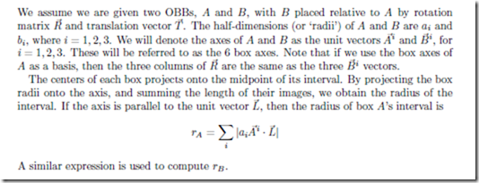
To perform the test, the algorithm projects the centers of the boxes onto the axis, and also to compute the radii of the intervals. If the distance between the box centers as projected onto the axis is greater than the sum of the radii, then the intervals (and the boxes as well) are disjoint. This is shown in 2D in Fig. 56.3.1.

OBB Representation and Overlap Test

All 15 axis tests simplify in similar fashion. Among all the tests, the absolute value of each element of R is used four times, so those expressions can be computed once before beginning the axis tests. If any one of the expressions is satisfied, the boxes are known to be disjoint, and the remainder of the 15 axis tests are unnecessary. This permits early exit from the series of tests. In practice, it takes up to 200 arithmetic operations in the worst case to check whether two OBBs overlap.

Implementation and Application

The OBBTree interference detection algorithm has been implemented and used as part of the following packages: RAPID, V-COLLIDE and PQP [12]. These implementations have been used for robot motion planning, dynamic simulation and virtual prototyping.

Performance of Bounding Volume Hierarchies

The performance of BVHs on proximity queries is governed by a number of design parameters. These include techniques to build the trees, number of children each node can have, and the choice of BV type. An additional design choice is the descent rule. This is the policy for generating recursive calls when a comparison of two BVs does not prune the recursion branch. For instance, if BVs A and B failed to prune, one may recursively compare A with each of the children of B, B with each of the children of A, or each of the children of A with each the children of B. This choice does not affect the correctness of the algorithm, but may impact the performance. Some of the commonly used algorithms assume that the BVHs are binary trees and each primitive is a single triangle or a polygon. The cost of performing the collision query is given as [27, 34]:

where T is the total cost function for collision queries, Nbv is the number of bounding volume pair operations, and Cbv is the total cost of a BV pair operation, including the cost of transforming and updating (including resizing) each BV for use in a given configuration of the models, and other per BV-operation overhead. Np is the number of primitive pairs tested for proximity, and Cp is the cost of testing a pair of primitives for proximity (e.g. overlaps or distance computation).

Typically for tight fitting bounding volumes, e.g., oriented bounding boxes (OBBs), Nbv and Np are relatively low, whereas Cbv is relatively high. In contrast, Cbv is low while Nbv and Np may be higher for simple BV types like spheres and axis-aligned bounding boxes (AABBs). Due to these opposing trends, no single BV yields optimum performance for collision detection in all possible cases.