Layout Data Structures:Corner Stitching

Corner Stitching

The corner stitching data structure was proposed by Ousterhout [8] to store non-overlapping rectilinear circuit components in MAGIC. The data structure is obtained by partitioning the layout area into horizontally maximal rectangular tiles. There are two types of tiles: solid and vacant, both of which are explicitly stored in the corner-stitching data structure. Tiles are obtained by extending horizontal lines from corners of all solid tiles until another solid tile or a boundary of the layout region is encountered. The set of solid and vacant tiles so obtained is unique for a given input. The partitioning scheme ensures that no two vacant or solid tiles share a vertical side. Each tile T is stored as a node which contains the coordinates of its bottom left corner, x1 and y1, and four pointers N , E, W , and S. N (respectively, E, W , S) points to the rightmost (respectively, topmost, bottommost, leftmost) tile neighboring its north (respectively, east, west, south) boundary. The x and y coordinates of the top right corner of T are T.E → x1 and T.N → y1, respectively, and are easily obtained in O(1) time. Figure 52.4 illustrates the corner stitching data structure.

The corner stitching data structure supports a rich set of operations.

1. Point Finding: given a tile T and a point p(x, y), search for the tile containing p by following a sequence of stitches starting at T .

2. Neighbor Finding: find all solid and vacant tiles that abut a given tile T .

3. Area Searches: determine whether any solid tiles intersect a given rectangular area R. This operation is used to determine whether a new solid tile can subse- quently be inserted into area R. (Recall that tiles in a layer are not permitted to overlap.)

4. Directed Area Enumeration: enumerate all the tiles contained in a given rectangular area in a specified order. This is used during the compaction operation which may require tiles to be visited and compacted in a left-to-right order.

5. Tile Creation: insert a solid tile T into the data structure at a specified location.

6. Tile Deletion: delete a specified solid tile T from the data structure.

7. Plowing: translate a large piece of a design. Move other pieces of the design that lie in its path in the same direction.

8. Compaction: this refers to one-dimensional compaction. We describe two operations to illustrate corner stitching:

Point Finding

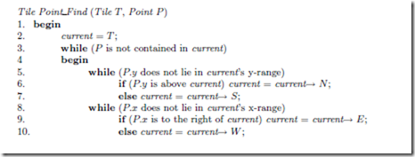
Next, we focus on the point find operation because of its effect on the performance of corner stitching. The algorithm is presented below. Given a pointer to an arbitrary tile T in the layout, the algorithm seeks the tile in the layout containing the point P .

Figure 52.5 illustrates the execution of the point find operation on a pathological example. From the start tile T , the while loop of line 5 follows north pointers until tile A is reached. We change directions at tile A since its y-range contains P . Next, west pointers are followed until tile F is reached (whose x-range contains P ). Notice that the sequence of west moves causes the algorithm to descend in the layout resulting in a vertical position that is similar to that of the start tile! As a result of this misalignment, the outer while loop of the algorithm must execute repeatedly until the point is found (note that the point will eventually be found since the point find algorithm is guaranteed to converge).

Tile Insertion

This operation creates a new solid tile and inserts it into the layout. It accomplishes this by a sequence of split and merge operations. The split operation breaks a tile into two tiles along either a vertical or a horizontal line. The merge operation combines two tiles to form a rectangular tile. Algorithm Insert discusses the insertion of a rectangle into the layout.

Insert(A) // (x1, y1 ) and (x2, y2 ) are the bottom left and top right corners of A.

1. if (!AreaSearch(A)) return; //area is not empty, abort.

2. Let i = 0; Split Qi, the tile containing the north edge of A into two tiles along the line y = y2 ; Let T be the upper tile and Qi be the lower tile.

3. while (Qi does not contain the south edge of A)

The rectangle A to be inserted is represented by thick, dashed lines in Figure 52.6(a). The coordinates of the bottom left and top right corners of A are (x1, y1) and (x2, y2), respectively. First, Step 1 of the algorithm uses AreaSearch to ensure that no solid tiles intersect A. Step 2 identifies tile Q0 as the vacant tile containing A’s north edge and splits it by the horizontal line y = y2 into two tiles: T above the split-line and Q0 below the split-line. Next, in the while loop of Step 3, Q0 is split by vertical lines at x1 and x2 to form L0, Q0, R0. Tile Q1 is the vacant tile below Q0. The resulting configuration is shown in Figure 52.6(b). In the next iteration, Q1 is split to form L1, Q1, and R1. L0 merges into L1 and Q0 merges into Q1. Tile Q2 is the vacant tile below Q1. The resulting configuration is shown in Figure 52.6(c). Next, Q2 is split to form L2, Q2, and R2. R1 is merged into R2 and Q1 merged into Q2. Figure 52.6(d) shows the configuration after Tile Q2 is processed. The vacant tile Q3 below Q2 contains R’s bottom edge and the while loop of Step 3 is exited. Steps 4, 5, and 6 of the algorithm result in the configuration of Figure 52.6(e). The final layout is shown in Figure 52.6(f).

Storage Requirements of the Corner Stitching Data Structure

Unlike simpler data structures such as arrays and linked lists, it is not trivial to manually estimate the storage requirements of a corner stitched layout. For example, if n items are inserted into a linked list, then the amount of storage required is n multiplied by the number of bytes required by a single list node. Because of vacant tiles, the total number of nodes in corner stitching is considerably more than n and depends on the relative positions of the n rectangles. In [9], a general formula for the memory requirements of the corner stitching data structure on a given layout. This formula requires knowledge about certain geometric properties of the layout called violations of the CV property and states that a corner stitching data structure representing a set of N solid, rectangular tiles with k violations contains 3N + 1 − k vacant tiles. Since each rectangular tile requires 28 bytes, the memory requirements are 28(4N + 1 − k) bytes.