Floorplan Representation in VLSI:Introduction and Graph Based Representations

Introduction

There are two main data models that can be used for representing floorplans: graph-based and placement based.

The graph-based approach includes constraint graphs, corner stitching, twin binary tree, and O-tree. They utilize constraint graphs or their simplified versions directly for the encoding. Constraint graphs are basic representations. The corner stitching simplifies the constraint graph by recording only the four neighboring blocks to each block. The twin binary tree then reduces the recorded information to only two neighbors of each block, and organizes the neighborhood relations in a pair of binary trees. The O-tree is a further simplification to the twin binary tree. It keeps only one tree for encoding.

The placement-based representations use the relative positions between blocks in a placement for encoding. This category includes sequence pair, bounded-sliceline grid, corner block list and slicing trees. The sequence pair and bounded-sliceline grid can be applied to general floorplan. The corner block list records only the relative position of adjacent blocks, and is available to mosaic floorplan only. The slicing trees are for slicing floorplan, which is a type of mosaic floorplan. The slicing floorplan can be constructed by hierarchical horizontal or vertical merges and thus can be captured by a binary tree structure known as the slicing tree.

The rest of this chapter is organized as follows. In Section 53.1, we give the introduction and the problem statement of floorplanning. In Section 53.2, we discuss the graph-based representations. In Section 53.3, we introduce the placement-based representations. We describe the relationship between different representations in Section 53.4. We illustrate the shape handling of rectilinear blocks in Section 53.5 and summarize the chapter in Section 53.6.

Statement of Floorplanning Problem

Today’s complexity in circuitry design wants a hierarchical approach [26]. The entire circuit is partitioned into several sub-circuits, and the sub-circuits are further partitioned into smaller sub-circuits, until they are small enough to be handled. The relationship between the sub-circuits can be represented with a tree as shown in Fig. 53.1. Here every sub- circuit is called a block, and hence the entire circuit is called the top block. From the layout point of view, every block corresponds to a rectangle, which contains sub-blocks or directly standard cells. Among the decisions to be made is the determination of shape (aspect ratio) and the pin positions on the blocks. In the top-down hierarchical methodology, blocks are designed from the top block (the entire circuit) to the leaf blocks (small modules). The minimizations of chip area and wire length are the basic targets for any layout algorithm. In addition, there are case-dependent constraints that will influence the layouts, such as the performance, the upper or/and lower boundaries of aspect ratio, the directions of pins, etc.

Now we give the definition of floorplanning problem: Inputs:

1. the net-lists of the sub-circuits;

2. the area estimation of blocks and, if any, the aspect ratio constraints on the blocks;

3. the target area and shape of the entire chip.

Outputs:

1. the shapes and positions of blocks;

2. the pin positions on the blocks.

The objective functions involve: the chip area, the total wire length and, if any, the performances.

Motivation of the Representation

Floorplan representation becomes an important issue in floorplanning for the following reasons.

(1) The blocks may have arbitrary shapes and locations, while the size of memory used to represent a two-dimensional floorplan should be O(n).

(2) For the general floorplanning problem, iterative improvement is the commonly used approach. The search for the best solution has proven to be NP-complete, so many heuristic optimizing algorithms, such as dynamic programming, simulated annealing, zone refine- ment, cluster refinement, have been adopted. The representation should also facilitate the operations called by those optimizing algorithms.

(3) The storage resources requirement, the redundancy of the representation and the complexity of translating the representation into floorplan are always the concerns in floor- planning. Here redundancy refers to the situation that several different expressions actually correspond to the same physical layout. Essentially, a heuristic algorithm searches part of the solution space to find the local optimal solution, which is hopefully very close to the global optimal solution. Redundancy causes the optimizing algorithm evaluate the same floorplan repeatedly.

Combinations and Complexities of the Various Representations

The number of possible floorplan representations describes how large the searching space is. It also discloses the redundancy of the representation. For general floorplans with n blocks, the combinations of the various representations are listed in Table 53.1. Note that the twin binary tree representation has a one to one relation with the mosaic floorplan, and the slicing tree has a one to one relation with the slicing floorplan [15]. In other words, for these two representations, the number of combinations is equal to the number of possible floorplan configurations and there is no redundancy.

The combination numbers of sequence pairs, mosaic floorplans, slicing floorplans, and O-trees are illustrated on a log scale in Fig. 53.2. The combination numbers are normalized by n!, which is the number of permutations of n blocks. The slopes of the lines for mosaic floorplans, slicing floorplans, and O-tree structures are the constants 0.89, 0.76, and 0.59, respectively. On the other hand, the slope of the line for sequence pair increases with a rate of log n.

Table 53.2 provides the exact numbers of the combinations for the floorplans or representations with the block number ranging from 1 to 17.

The time complexities of the operations transforming a representation to a floorplan are

very important, because they determine the efficiency of the floorplan optimizations. The complexities of the representations covered in this chapter are compared in Table 53.3, where n is the number of blocks in a floorplan.

For sequence-pair, the time complexity to derive a floorplan is O(nloglogn) due to a fast algorithm proposed in [8]. We will discuss more on this in Section 53.3.1 For bounded slicing grid, there is a trade off between the solution space and the time complexity of deriving a floorplan. To ensure that the solution space covers all the optimal solutions, we need the grid size to be at lease n by n. This results in an O(n2) time complexity in deriving a floorplan [6]. For the rest of the representations, there are algorithms with O(n) time complexity to convert them into constraint graphs. The time complexity to derive a floorplan is thus O(n).

Slicing, Mosaic, LB Compact, and General Floorplans

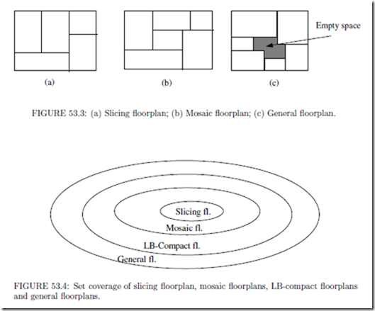
A layout can be classified as a slicing floorplan if we can partition the chip with recursive horizontal or vertical cut lines (Fig. 53.3(a)). In a mosaic floorplan, the chip is partitioned by horizontal and vertical segments into rectangular regions and each region corresponds to exactly one block (Fig. 53.3(b)). For a general floorplan, we may find empty space outside rectangular block regions (Fig. 53.3(c)). An LB-compact floorplan is a restricted general floorplan in that all blocks are shifted to their left and bottom limits. In summary, the set of general floorplans covers the set of LB-compact floorplans, which covers the set of mosaic floorplans, and which covers the set of slicing floorplans (Fig. 53.4).

For slicing and mosaic floorplans, the vertical segments define the left-right relation among the separated regions, and the horizontal segments define the above-below relation. Suppose that we shift the segments to change the sizes of the regions, we view the new floorplan to be equivalent to the original floorplan in terms of their topologies[4][23][24]. Therefore, we can devise representations to define the topologies of slicing and mosaic floorplans independent of the sizes of the blocks (Fig. 53.3(a) and (b)). In contrast, for a general floorplan, it is rather difficult to draw a meaningful layout (Fig. 53.3(c)) without the knowledge of the block dimensions. One approach is to extend the mosaic floorplans to general floorplans by adding empty blocks [16]. It is shown that to convert a mosaic floorplan with n blocks into a general floorplan, the upper bound on the number of empty blocks inserted is n − 2√n +1. [16]

In a mosaic floorplan, two adjacent blocks meet at a T-junction by sharing the non- crossing edge of the junction. There are four directions of T-junctions as is illustrated in Fig. 53.5. In the case of Fig. 53.5(a) and (b), block B is termed the C-neighbor at the lower left corner of block A. In Fig. 53.5(c) and (d), block B is the C-neighbor at the upper right corner of block A. The C-neighbor is used to construct twin binary tree representation.

The degeneration of a mosaic floorplan refers to the phenomenon that two T-junctions meet together to make up a cross-junction, as illustrated in Fig. 53.6(a). Some representations forbid the occurrence of degeneration. One scheme to solve the problem is to break one of the intersecting lines and assume a slight shift between the two segments, as shown in Fig. 53.6(b). Thus the degeneration disappears.

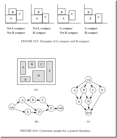
We generate an LB compact floorplan by compacting all blocks toward left and bottom. For a placement, suppose no block can be moved left, the placement is called L-compact. Similarly, if no block can be moved down, the placement is called B-compact. A floorplan is LB-compact if it is both L-compact and B-compact (Fig. 53.7).

Graph Based Representations

Graph based representations include constraint graphs, corner stitching, twin binary trees, and O-tree. They all utilize the constraint graphs or their simplified version for floorplan encoding.

Constraint Graphs

Constraint graphs are directed acyclic graphs representing the adjacency relations between the blocks in a floorplan. In this subsection, we first define the constraint graphs for general floorplans. We then show that for mosaic floorplan, the constraint graphs have nice properties of triangulation and duality.

The generation of constraint graphs

Constraint graphs reflect the relative positions between blocks [12]. Constraint graphs can be applied to general floorplans, as is shown in Fig.53.8. A node in the constraint graph represents a block. A directed edge denotes the location relationship between two blocks. For example, A→B means block A is to the left of B in a horizontal constraint graph (Fig. 53.8(b)). A→E means block A is on top of E in a vertical constraint graph (Fig. 53.8(c)).

Here we imply that if A→B and B→C, then A→C. Thus even though block A stands to the left of C, the edge between A and C is not necessarily shown. To mark the four sides of the chip, we add the nodes labeled with “left”, “right”, “top” and “down”. A pair of horizontal and vertical constraints graphs can represent a floorplan. Every constraint graph, whether it is a horizontal one or a vertical one, is plan r and acyclic. Fig. 53.9 shows an example of the constraint graphs to a mosaic floorplan. Fig 53.9(a) is the mosaic floorplan. Fig 53.9(b) and (c) are the corresponding horizontal and vertical constraint graphs, respectively.

Triangulation

For a mosaic floorplan without degeneration, if its horizontal and vertical constraint graphs are merged together, then we have the following conclusions [12]:

1. Every face is a triangle.

2. All internal nodes have a degree of at least 4.

3. All cycles, if not faces, have the length of at least 4.

Shown in Fig. 53.10(a) is the result of merging the pair of constraint graphs in Fig. 53.9. In fact, the merged constraint graph is a dual graph of its original floorplan (Fig. 53.9(b)).

Tutte’s duality[27]

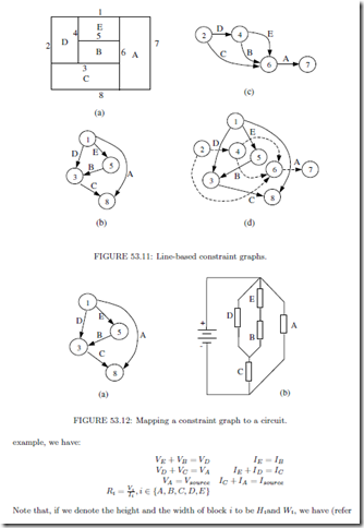
We can also build an edge-based constraint graph for a mosaic floorplan, where the nodes denote the lines separating the blocks while the edges denote the blocks. Labeling the lines with numbers (Fig. 53.11(a)), we build a vertical constraint graph (Fig. 53.11 (b))

and a horizontal constraint graph (Fig. 53.11(c)). Fig. 53.11(d) demonstrates the result of merging the vertical and horizontal constraint graphs. Here, to make the merged graph clear, the edges representing horizontal constraints are drawn with dotted lines, and a letter at the intersection of a solid edge and a dotted edge denotes the two edges simultaneously. It is very interesting that, for mosaic floorplans, the vertical and horizontal constraint graphs are dual, as is called Tutte’s duality.

Let’s see how Tutte’s duality is used to solve the sizing problem in floorplanning. We map the constraint graphs into circuit diagrams by replacing the edges in the vertical constraint graph with resistors, as illustrated in Fig. 53.12.

The circuit is subject to Kirchoff voltage law. As a result, taking Fig. 53.12 as an

By comparing the above two equation arrays, we can find that there is a perfect correspondence between the solutions of the circuit and the floorplan. Let us set the following assumptions: (only two of the three equations are independent)

Thus the theories dealing with large circuits can be borrowed to solve the sizing problem in floorplanning.

Constraint graphs have the advantages of being able to cope with any types of floorplans. However, it would be rather difficult to shift to a new floorplan with just a few simple operations on the graph. The efficiency is greatly discounted for the iteratively improving algorithms. Thus in [25], a transitive closure graph (TCG) was proposed to simplify the rules of the operations. The relation of each pair of blocks is prescribed in either horizontal or vertical constraint graph via transitive closure, but not in both graphs.

Corner Stitching

Corner stitching is used to represent the topology of a mosaic floorplan. Simplified from constraint graphs, corner stitching [17] keeps only four pointers at the two opposite corners for every block. All the operations on a constraint graph can also be fulfilled on a corner stitching representation with acceptable increases in time complexity, while the storage for corner stitching becomes easier since the number of pointers attached to every block is fixed (equals to 4). Readers are referred to Chapter 52 for detailed descriptions and analyses of corner stitching.

Twin Binary Tree

Twin binary tree [15] representation applies to mosaic floorplans without degeneration. The twin binary tree is constructed as follows, every block takes its C-neighbor (Fig. 53.5) as its parent. In the first tree, only the C-neighbors in lower left corners (Fig. 53.5 (a) and (b)) are taken into account. If the related T-junction is of type (a), then the block is a left child of its parent, and if the T-junction is of type (b), then the block is a right child. The most bottom-left block in the floorplan acts as the root of the tree. Similarly, in the second tree, the C-neighbors in upper right corners (Fig. 53.12(c) and (d)) are used, and the most upper-right block becomes the tree’s root.

tree.Fig.53.13 gives an example of a twin binary The pointers of twin binary trees are in fact a subset of those in corner stitching. Besides, It has been proved that twin binary tree is a non-redundant representation. In other words, every pair of trees corresponds to a unique mosaic floorplan.

The twin properties of binary trees can be illustrated with Fig. 53.14. Consider the trees shown in Fig. 53.13, we add a left child labeled ‘0’ to every node without left child except the most left node, and a right child labeled ‘1’ to every node without right child except the most right node. The resultant trees are the so-called extended trees (Fig. 53.14). The sequences of the in-order traverse of the two extended trees shown in Fig. 53.14 are “A0B1C1F0D1E” and “A1B0C0F1D0E” respectively. If we separate them into the label parts and the bit parts, we have π1=ABCFDE, α1=01101 π2= ABCFDE and α2 = 10010. It is interesting to find that π1=π2 and α1 = α2. So rather than store the two binary trees, we only keep the linear listsπ andαin memory.

However, it is insufficient to recover the two binary trees just from π and α, so we need two more lists, β and βI . If the i-th element inπ is the left child of its parent in the first tree or the root of the tree, we set the i-th element in β to be ‘0’, otherwise we set it ‘1’. In the

similar way βI is constructed according to the second tree. Thus we use a group of linear lists {π,α, β,βI }, called the twin binary sequence [16], to express the twin binary tree, and equivalently the floorplan.

Finally, we give the main properties of twin binary tree representation:

1.The memory required for storing the twin binary sequence is log2n+3n-1, because |π|= log2n, |α| = n-1, and |β| = |β | = n.

2. Twin binary tree is a non-redundancy floorplan representation.

3. The complexity of the translation between twin binary sequence and floorplan is O(n).

Single Tree Representations

An ordered-tree (O-tree) [2][3], or equivalently the B∗ tree [1] representation uses a spanning tree of the constraint graph and the dimensions of the blocks. Because the widths and heights of the blocks are given, the representation can describe one kind of general floorplan termed LB-compact. With a proper encoding, a great enhancement on the storage efficiency and the perturbation easiness is obtained.

A horizontal O-tree is derived with the following rules:

1. If block A lies adjacent to the left side of block B, or, Xa + Wa = Xb (here Xa is the coordinate of block A on the X-axis and Wa is the width of block A), then on the O-tree, B is A’s child. If there happens to exist more than one block adjacent to the left side of block B (satisfying the requirement Xi + Wi = Xb), one of them is assigned to be the parent of block B.

2. If block A lies on top of block B and the two blocks have the same parents on the O-tree, then B is A’s elder brother.

3. A virtual block is presumed to have the left most position, and therefore serves as the root of the O-tree.

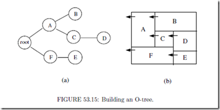
Fig. 53.15 shows an example of an O-tree representation for the same mosaic floorplan shown in Fig. 53.13.

If we show the pointer of every block pointing to its parent in the O-tree (Fig. 53.15(b)), we can find that the pointers are in fact a subset of those in twin binary tree. Similarly a vertical O-tree can be built up. Without the loss of generality, hereafter we only discuss the horizontal O-tree.

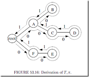
Next, let’s describe the O-tree with linear lists: a bit string (denoted with T ) and a label string (denoted with π). The bit string records the structure of an O-tree. We make a depth-first traverse on the O-tree. A “0” is inserted into T for descending an edge while a “1” for ascending an edge. For example, the O-tree in Fig. 53.16 corresponds to the bit string T=“001100011011”. Inversely, given the bit string, the structure of the O-tree is solely determined. To get the complete description of an O-tree, we need a second linear list, the label string, to record the labels of the tree’s nodes. Not only should the label string include all the labels of the tree’s nodes, but also reflect the labels’ positions on the tree. A depth-first traverse generates such a linear list. For the example in Fig. 53.16, we have π= ‘FEACDB’.

Given a horizontal O-tree, or {T, π}, and the dimensions of blocks, the positions of blocks can be derived with the following rules:

1. Each block has to be placed to the left of its children.

2. If two blocks overlap along their x-coordinate projection, then the block having a higher index in π must be placed on top of the other one.

In fact the second rule applies to the situation in which none of the two blocks is a descendant of the other, like blocks ‘f ! and “a”, or “b” and “d”, in Fig. 53.16. The way we derive π indicates that the block with higher index always stands “higher”. To get to a placement, we need to locate all the blocks. The following operation is executed on blocks according to their orders in π. Here Bi refers to the i-th block, and (xi, yi) refers to the coordinate of Bi’s left-bottom corner.

1. Find Bi’s parent, Bj , and then we havexi = xj + wj , here wj is the width of block Bj .

2. Let ψ be a set of blocks who have a lower index than Bi in π and have an projection overlap with Bi in the X-axis, find the maximum yk + wk for Bk ∈ ψ, then we have yi = max(yk + wk ).

Now we analyze the performance of O-tree:

1. The bit string has a length of 2n for an O-tree of n blocks, because each node except the root has an edge towards its parents and each edge is traversed twice during the construction of the bit string. The label string takes n log2 n bits for we have to use log2 n bits to distinguish the n blocks. So the total memory occupied by an O-tree is n(2 + log2 n). By comparison, a sequence pair takes 2n log2 n bits and a slicing structure takes n(6 + log2 n) bits.

2. The time needed to transform {T,π} to a placement is linear to the number of blocks, or we can say the complexity of transforming {T,π} to a placement is O(n). For a sequence pair or a slicing structure, the complexity is O(n log2 log2n) or O(n) respectively. Upon this point, O-tree has the same performance as the slicing structure but is more powerful for representing a placement.

3. The number of combinations is O(n!·22n−2/n1.5), which is smaller than any other representation that has ever been discussed.

The floorplan of an arbitrarily given O-tree is not necessarily LB-compact. Yet in this case, we can compact the floorplan to reduce the chip area. Notice that an O-tree-to- placement transform tightens the blocks, with one direction having the priority. For ex- ample, in a placement transformed from a horizontal O-tree, the blocks are placed tighter along the X-axis than along the Y-axis. It would be undoubted that a placement trans- formed from a vertical O-tree will give Y-axis the priority. Thus, by iteratively making the transforms between horizontal O-trees and vertical O-trees via placements, we can finally reach an LB-compact floorplan (Fig. 53.17).

On the other hand, given an LB-compact floor plan, we can always derive an O-tree representation. For example, Figure 53.18 illustrates a general floor plan with seven blocks and the corresponding O-tree. O-tree is able to cover LB-compact floor plan with the smallest number of combinations in Table 53.1 and Fig. 53.2 because the O-tree structure avoids redundancy and screens improper floor plans by taking advantage of the knowledge of the block dimensions. For example, given an O-tree, we can convert it to a binary tree and find many other possible trees to pair up as twin binary trees, which correspond to many different mosaic floorplans. In the perspective of O-tree representation, these floorplans are the variations due to the differences of the block sizes.

The B∗ tree and the O-tree are equivalent because the transformation between the two is one to one mapping. The merit of the B tree is a different data structure and implementation.

In summary, among the constraint-graphs based representations, from the point of view of the pointers necessary for representing the floor plans, O-tree is a subset of twin binary tree; twin binary is a subset of corner stitching; and corner stitching is a subset of constraint graphs, as demonstrated in Fig. 53.19.