Drawing Trees:Level Layout for n-ary Trees

Level Layout for n-ary Trees

A straightforward manner to draw trees of unbounded degree is to adjust the Rein gold Tilford algorithm by traversing the children of each node v from left to right, successively computing the preliminary coordinates and the modifiers.

This however violates property (A5): the subtrees are placed as close to each other as possible and small subtrees between larger ones are piled to the left; see Figure 45.3(a). A simple trick to avoid this effect is to add an analogous second traversal from right to left; see Figure 45.3(b), and to take average positions after that. This algorithm satisfies (A1) to (A5), but smaller subtrees are usually clustered then; see Figure 45.3(c).

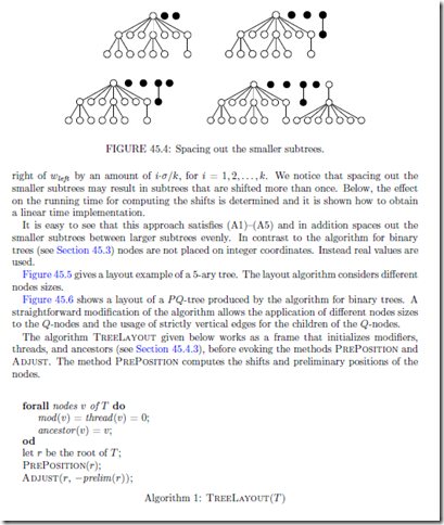
To obtain a layout where smaller subtrees are spaced out evenly between larger subtrees as for example shown in Figure 45.3(d), we process the subtrees for each node v ∈ V from left to right, see Figure 45.4. In a first step, every subtree is then placed as close as possible to the right of its left subtrees. This is done similarly to the algorithm for binary trees as described in Section 45.3 by traversing the left contour of the right subtree T (wright ) and the right contour of the subforest induced by the left siblings of wright .

Whenever two conflicting neighbors vleft and vright are detected, forcing vright to be shifted to the right by an amount of σ, we apply an appropriate shift to all smaller subtrees between the subtrees containing vleft and vright .

More precisely, let wleft and wright be the greatest distinct ancestors of vleft and vright . Notice that both wleft and wright are children of the node v that is currently processed. Let k be the number of children w1, w2,..., wk of the current root between wleft and wright + 1. The subtrees between wleft and wright are spaced out by shifting the subtree T (wi) to the

Based on the results of the function PrePosition the function Adjust given in Algo- rithm 2 computes the final coordinates by summing up the modifiers recursively.

PrePosition

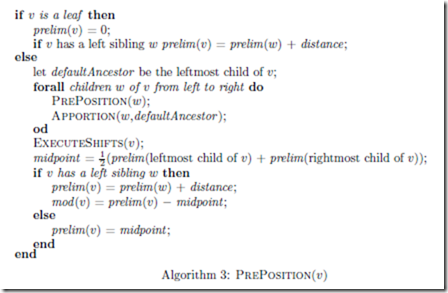
Algorithm 3 presents the method PrePosition(v) that computes a preliminary x-coordinate for a node v. PrePosition is applied recursively to the children of v. After each call

of PrePosition on a child w a function Apportion is executed on w. The procedure Apportion is the core of the algorithm and shifts a subtree such that it does not conflict with its left subforest. After spacing out the smaller subtrees by calling Execute Shifts, the node v is placed to the midpoint of its outermost children. The value distance pre- scribes the minimal distance between two nodes. If objects of different size are considered for the representation of the nodes, or if different minimal distances, i.e. between subtrees, are specified, the value distance has to be modified appropriately.

Combining a Subtree and Its Left Subforest

Before presenting Apportion in detail, we need to consider efficient strategies for the different tasks that are performed by this function.

Similar to the threads used for binary trees (see Sect. 45.3), Apportion uses threads to follow the contours of the right subtree and the left subforest. The fact that the left subforest is no tree in general does not create any additional difficulty.

One major task of Apportion is that it has to space out the smaller subtrees between the larger ones. More precisely, if Apportion shifts a subtree to the right to avoid a conflict with its left subforest, Apportion has to make sure that the shifts of the smaller subtrees of the left subforest are determined.

A straightforward implementation computes the shifts for the intermediate smaller sub- trees after the right subtree has been moved. However, as has been shown in [2], this strategy has an aggregated runtime of Ω(|V 3/2 ). To prove this consider a tree T k such that the root has k children v1, v2,... , vk (see Figure 45.7 for k = 3). The children are numbered from left to right. Except for v1 let the i-th child vi be the root of a subtree T k(vi) that consist of a chain of i nodes. Between each pair vi, vi+1, i = 1, 2,... ,k − 1, of these children, add k children as leaves. Moreover, the subtree T k(v1) is modified as follows. Its root v1 has 2k + 5 children, and up to level k − 1, every rightmost child of the 2k + 5 children again

The next Section 45.4.3 shows how to obtain the tree T (vj ) efficiently. Section 45.4.4 gives a detailed description on how to compute the shift of T (vi) and Section 45.4.5 presents a method that spaces out smaller subtrees.

Ancestor

We first describe how to obtain the subtree T (vj ) that contains the node vleft . The problem is equivalent to finding the greatest distinct ancestors wleft and wright of the nodes vleft and vright , where in this case wleft is equal to the root vj of the subtree that we need to determine and wright = vi. It is possible to apply an algorithm by Schieber and Vishkin [19] that determines for each pair of nodes its greatest distinct ancestors in constant time, after an O(|V |) preprocessing step. Since their algorithm is somewhat tricky, and one  of the greatest distinct ancestors, namely vi, is known anyway, we apply a much simpler algorithm. Furthermore, as vright is always the right neighbor of vleft , the left one of the greatest distinct ancestors only depends on vleft . Thus we may shortly call it the ancestor of vleft in the following.

FIGURE 45.8: Adjusting ancestor pointers when adding new subtrees: the pointer ancestor (u) is represented by a solid arrow if it is up to date and by a dashed arrow if it has expired. In the latter case, the defaultAncestor is used and drawn black. When adding a small subtree, all ancestor pointers ancestor (u) of its right contour are updated. When adding a large subtree, only defaultAncestor is updated.

To store the ancestor of a node u a pointer ancestor (u) is introduced and initialized to u itself. The pointer ancestor (u) for any node u is not updated throughout the algorithm. Instead, a defaultAncestor is used and ancestors are only determined for the nodes u on the

Apportion

Shifting the Smaller Subtrees

For spacing out the smaller subtrees evenly, the number of the smaller subtrees between the larger ones has to be maintained. Since simply counting the number of smaller children between two larger subtrees T (vj ) and T (vi), 1 ≤ j < i ≤ k would result in Ω(n3/2) time in total, it is determined as follows. The children of v are numbered consecutively. Once the pair of nodes vleft , vright that defines the maximum shift on T (vi) has been determined, the greatest distinct ancestors wleft = vj and wright = vi are easily determined by the approach described in Section 45.4.3. The number i − j − 1 gives the number of in between subtrees in constant time.

1. the value shift (vi ) is increased by σ

2. the value change(vi ) is decreased by σ/θ

3. the value change(vj ) is increased by σ/θ

Figure 45.9 shows an example on setting the values of shift () and change(). By construction of the arrays shift () and change() we then obtain the shift of T (vg ), g = 1, 2,... , k, (including the “original” shift of the subtree T (vi)) as follows. The children vg , g = k, k − 1,... , 1, are traversed from right to left. Two real values σ and change are maintained to store the shifts and the decreases of shift per subtree, respectively. These values are initialized with zero. When visiting child vg , g ∈ {k, k−1,... , 1} the subtree T (vg ) is shifted to the right by σ (i.e., we increase prelim(vg ) and mod (vg ) by σ). Furthermore, change is increased by change(vg ), and σ is increased by shift (vg ) and by change(vg ) and we continue with vg−1.

The function ExecuteShifts(v) traverses its children from right to left and determines the total shift of the children based on the arrays shift () and change().

THEOREM 45.2 [Buchheim et al. [2]] The layout algorithm for n-ary trees meets the aes- thetic requirements (A1)–(A5), spaces out smaller subtrees evenly, and can be implemented to run in O(|V |).

Proof By construction of the algorithm it is obvious that the algorithm meets (A1)–(A5) and spaces out the smaller subtrees evenly. So it is left to show that the running time is linear in the number of nodes.

Every node of T is traversed once during the traversals PrePosition and Adjust.

Similar reasoning as in the proof of theorem 45.1 for binary trees shows that the time needed to traverse the left contour of the subtree T (vi) and the right contour of subforest ∪h=1T (vh), i = 2, 3,... ,k for every node v with children vi, i = 1, 2,... ,k is linear in the number of nodes of T over all such traversals. Moreover, we have that by construction the number of extra operations for spacing out the smaller subtrees is linear in |V | plus the number of nodes traversed in the contours. This proves the theorem.