LEDA, a Platform for Combinatorial and Geometric Computing:Example Programs
In this section we give several programming examples showing how Leda can be used to implement combinatorial and geometric algorithms in a very elegant and readable way. In each case we will first state the algorithm and then show the program. It is not essential to understand the algorithms in full detail; our goal is to show:
• how easily the algorithms are transferred into programs and
• how natural and elegant the programs are.
Algorithm + Leda = Program.
Word Count
We start with a very simple program. The task is to read a sequence of strings from standard input, to count the number of occurrences of each string in the input, and to print a list of all occurring strings together with their frequencies on standard output.
The program uses the Leda types string and d array (dictionary arrays). The parameterized data type d array<I , E > realizes arrays with index type I and element type E. We use it with index type string and element type int .
We give some more explanations. The program starts with the include statement for dictionary arrays and skip lists. In the first line of the main program we define a dictionary array N with index type string, element type int and implementation skip list and initialize all entries of the array to zero. Conceptually, this creates an infinite array with one entry for each conceivable string and sets all entries to zero; the implementation of d arrays stores the non-zero entries in a balanced search tree with key type string. In the second line we define a string s. The while-loop does most of the work. We read strings from the standard input
FIGURE 41.3: A shortest path in a graph. Each edge has a non-negative cost. The cost of a path is the sum of the cost of its edges. The source node s is indicated as a square. For each node the length of the shortest path from s is shown.
until the end of the input stream is reached. For every string s we increment the entry N [s] of the array N by one. The iteration forall defined (s, N ) in the last line successively assigns all strings to s for which the corresponding entry of N was touched during execution. For each such string, the string and its frequency are printed on the standard output.
Dijkstra’s shortest path algorithm [7] takes a directed graph G = (V, E), a node s ∈ V , called the source, and a non-negative cost function on the edges cost : E → R≥0. It computes for each node v ∈ V the distance from s, see Figure 41.3. A typical text book presentation of the algorithm is as follows:
The text book presentation will then continue to discuss the implementation of line (*). It will state that the pairs {(v, dist (v)); v unreached} should be stored in a priority queue, e.g., a Fibonacci heap, because this will allow the selection of an unreached node with minimal distance value in logarithmic time. It will probably refer to some other chapter of the book for a discussion of priority queues.
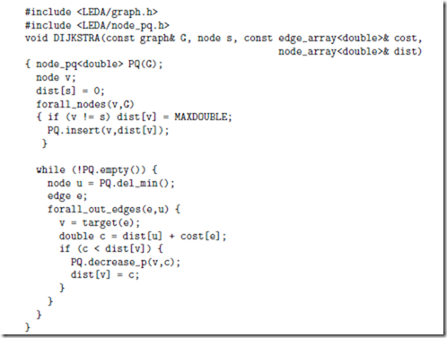
We next give the corresponding Leda program; it is very similar to the pseudo-code above. In fact, after some experience with Leda you should be able to turn the pseudo code into code within a few minutes.
We start by including the graph and the node priority queue data types. The function DIJKSTRA takes a graph G, a node s, an edge array cost , and a node array dist . Edge arrays and node arrays are arrays indexed by edges and nodes, respectively. We declare a priority queue PQ for the nodes of graph G. It stores pairs (v, dist [v]) and is initially empty. The forall nodes -loop initializes dist and PQ . In the main loop we repeatedly select a pair (u, dist [u]) with minimal distance value and then iterate over all out-going edges to update distance values of neighboring vertices.
We next incorporate the shortest path program into a small demo. We generate a random graph with n nodes and m edges and choose the edge costs as random number in the range [0, 100]. We call the function above and report the running time.
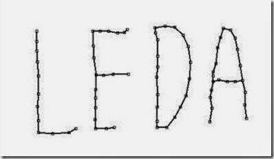
The reconstruction of a curve from a set of sample points is an important problem in computer vision. Amenta, Bern, and Eppstein [2] introduced a reconstruction algorithm which they called CRUST. Figure 41.4 shows a point set and the curves reconstructed by their algorithm. The algorithm CRUST takes a list S of points and returns a graph G. CRUST makes use of Delaunay diagrams and Voronoi diagrams and proceeds in three steps:
• It first constructs the Voronoi diagram VD of the points in S.
• It then constructs a set L = S ∪ V , where V is the set of vertices of VD .
• Finally, it constructs the Delaunay triangulation DT of L and makes G the graph of all edges of DT that connect points in S.
The algorithm is very simple to implement
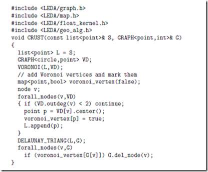
We give some explanations. We start by including graphs, maps, the floating point geometry kernel, and the geometry algorithms. In CRUST we first make a copy of S in L. Next we compute the Voronoi diagram VD of the points in L. In Leda we represent Voronoi diagrams by graphs whose nodes are labeled with circles. A node v is labeled by a circle passing through the defining sites of the vertex. In particular, VD [v].center ( ) is the position of the node v in the plane. Having computed VD we iterate over all nodes of VD and add all finite vertices (a Voronoi diagram also has nodes at infinity, they have degree one in our graph representation of Voronoi diagrams) to L. We also mark all added points
FIGURE 41.4: A set of points in the plane and the curve reconstructed by CRUST. The figure was generated by the program presented in Section 41.6.3.
as vertices of the Voronoi diagram. Next we compute the Delaunay triangulation of the extended point set in G. Having computed the Delaunay triangulation, we collect all nodes of G that correspond to vertices of the Voronoi diagram in a list vlist and delete all nodes in vlist from G. The resulting graph is the result of the reconstruction.
We next incorporate CRUST into a small demo which illustrates its speed. We generate n random points in the plane and construct their crust. We are aware that it does really make sense to apply CRUST to a random set of points, but the goal of the demo is to illustrate the running time.
We give some more explanations. We start by including the window type. In the main program we define a window and open its display. A window will pop up. We state that we want nodes and edges to be drawn with width two. We define the list S and the graph G required for CRUST. In each iteration of the while-loop we read a point in W (each click of the left mouse button enters a point), append it to S and compute the crust of S in G. We then draw G by drawing its vertices and its edges. Each edge is drawn as a line segment connecting its endpoints. Figure 41.4 was generated with the program above.
In the next example we show how to use Leda for computing the upper convex hull of a given set of points. The following function UPPER HULL takes a list L of rational points (type rat point) as input and returns the list of points of the upper convex hull of L in clockwise ordering. The algorithm is a variant of Graham’s Scan [25]. First we sort L according to the lexicographic ordering of the Cartesian coordinates and remove multiple points. If the list contains not more than two points after this step we stop. Before starting the actual Graham Scan we first skip all initial points lying on or below the line connecting the two extreme points. Then we scan the remaining points from left to right and maintain the upper hull of all points seen so far in a list called hull. Note however that the last point of the hull is not stored in this list but in a separate variable p. This makes it easier to access the last two hull points as required by the algorithm. Note also that we use the rightmost point as a sentinel avoiding the special case that hull becomes empty.
Leda represents triangulations by bidirected plane graphs (from the graph library) whose nodes are labeled with points and whose edges may carry additional information, e.g. integer flags indicating the type of edge (hull edge, triangulation edge, etc.). All edges incident to a node v are ordered in counter-clockwise ordering and every edge has a reversal edge. In this way the faces of the graph represent the triangles of the triangulation. The graph type offers methods for iterating over the nodes, edges, and adjacency lists of the graph. In the case of plane graphs there are also operations for retrieving the reverse edge and for iterating over the edges of a face. Furthermore, edges can be moved to new nodes. This graph operation is used in the following program to implement edge flips.
Function DELAUNAY FLIPPING takes as input an arbitrary triangulation and turns into a Delaunay triangulation by the well-known flipping algorithm. This algorithm performs a sequence of local transformations as shown in Figure 41.5 to establish the Delaunay property: for every triangle the circumscribing sphere does not contain any vertex of the triangulation in its interior. The test whether an edge has to be flipped or not can be realized by a so-called side of circle test. This test takes four points a, b, c, d and decides on which side of the oriented circle through the first three points a,b, and c the last point d lies. The result is positive or negative if d lies on the left or on the right side of the circle, respectively, and the result is zero if all four points lie on one common circle. The algorithms uses a list of candidates which might have to be flipped (initially all edges). After a flip the four edges of the corresponding quadrilateral are pushed onto this candidate list. Note that G[v] returns the position of node v in the triangulation graph G. A detailed description of the algorithm and its implementation can be found in the Leda book ([27]).
Discussion
In each of the above examples only a few lines of code were necessary to achieve complex functionality and, moreover, the code is elegant and readable. The data structures and algorithms in Leda are efficient. For example, the computation of shortest paths in a graph with 10000 nodes and 100000 edges and the computation of the crust of 5000 points takes less than a second each. We conclude that Leda is ideally suited for rapid prototyping as summarized in the equation Algorithm + Leda = Efficient Program.


Comments
Post a Comment